In the previous notebook, we saw that adding flexibility to a model improves its ability to approximate complex relationships. Additional flexibility also increases the model’s ability to fit the training data – that is, more flexible models will generally have lower training error than less flexible models. Because training error continues to drop with additional flexibility, we need an additional data source which was unseen by the model during the training process in order to provide an unbiased estimate of future model performance. Ideally, this test error will decrease until the optimal level of model flexibility is reached but then the test error will increase once the model becomes overfit to the training data.
At the end of the last notebook, we drew an elbow plot, showing how the training and test errors changed as model flexibility was increased. This visual technique allowed us to identify which models were likely underfit and what the threshold for an overfit model was. We can use these elbow plots in general, to identify an appropriate level of flexibility for our models.
Motivation
We’ve placed a lot of faith in our training and test sets over the last few weeks. We’ve given the training data total power to determine our model coefficients and the test data sole power to determine our expected performance metrics (R-Squared, RMSE, etc.). Perhaps we should have some concern here – especially given our most recent discussion about model flexibility and its relationship to variance. Different training data would result in differently estimated coefficients and different testing data would result in differently estimated performance estimates – do we really want to believe that our random data splitting resulted in perfectly fair and representative training and test data? It is certainly possible that we, by chance, would generate a particularly “easy” training set and a particularly “difficult” test set (or vice-versa). Furthermore, if we are in the business of constructing models often, such an occurrence is guaranteed eventually!
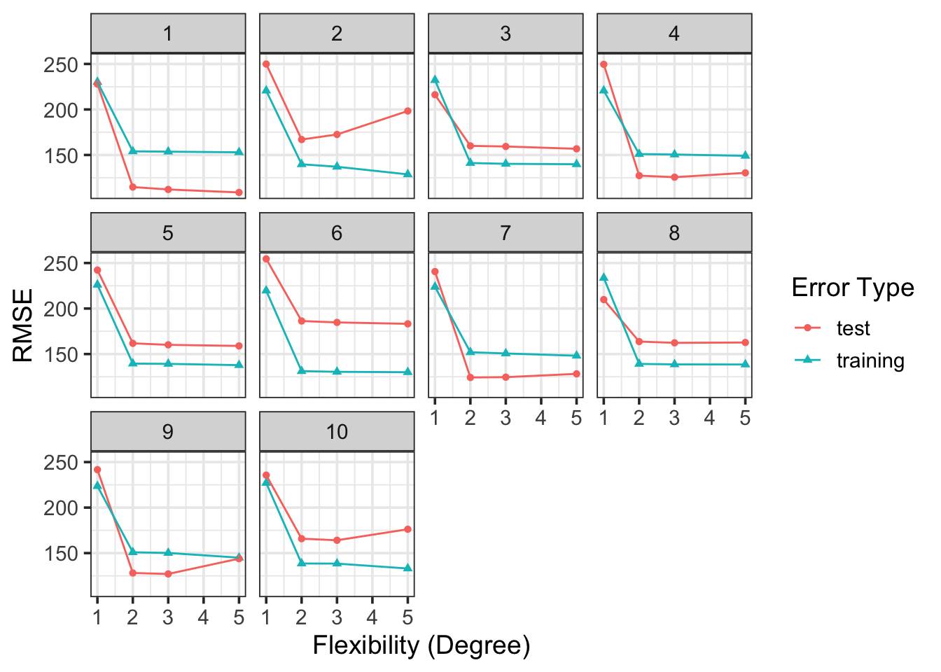
To highlight how much influence our training and test sets can have on our models and the expectations we develop about them, each plot below corresponds to the RMSE for models of degree \(1\), \(2\), \(3\), and \(5\) for a single data set but using a different training/testing splits. To produce the plots below, I’ve generated a toy dataset and am constructing/analyzing the performance of a variety of models (linear, quadratic, cubic, fifth-degree) for 10 different training/test set combinations below. Interpret the elbow plots to see how the estimated performance metrics change for each different training and test set.
The elbow plots pretty reliably identify the appropriate level of model flexibility. In the toy data set I generated, the true association between \(x\) and \(y\) was quadratic. However, the test RMSE, which we utilize in estimating the “accuracy” of our model’s predictions fluctuates quite wildly – between a low of below \(115\) for the first training/test set combination, and a high of nearly \(190\) for the sixth training/test combination. There is a big difference between claiming our model’s typical prediction error will be on the order of \(115\) units and on the order of \(190\) units. These discrepancies should be worrisome. We are putting lots of trust in our models, so it would be nice to have more certainty about our estimated coefficients, predictions, and error/performance estimates.
Objectives
The discussions above have highlighted that, while we thought we were doing the right things with our training and test set approach all along, we were actually very vulnerable to the random data that – by chance – fell into our training set and our test set. Different splits can lead to different models and certainly different model performance expectations. In this notebook, we’ll develop a robust framework which will help us obtain more reliable performance estimates and help us estimate how uncertain we are in those estimates.
After working through this notebook you should be able to:
Describe the pitfalls associated with the validation set approach we’ve been using up to this point in our course.
Describe how cross-validation works as well as how it mitigates the issues associated with a single validation set.
Implement cross-validation using vfold_cv() in conjunction with fit_resamples() from {tidymodels} to fit and assess models using cross-validation.
Observe and interpret individual performance metrics on each cross-validation fold as well as to aggregate those metrics to a more stable performance estimate along with an estimate for our uncertainty in this metric.
Cross-Validation
In cross-validation, rather thank breaking our data set into a single training and test set, we’ll break our data into \(k\) folds, were \(k\) is somewhere between \(3\) and \(n\) (your total number of observations). Each of the folds will take one turn playing the role of the test set for a model fit on all of the other folds – that is, with cross-validation, we’ll fit \(k\) models and get \(k\) performance estimates. Once we have those performance estimates, they can be averaged and we can compute the standard error corresponding to the performance metric. This provides us (i) more stable and reliable model performance estimates, and (ii) a way to quantify the uncertainty associated with those metrics.
The most commonly utilized number of folds are \(5\) and \(10\). In the special case where you utilize \(n\) folds, each observation belongs to its own fold – this is often called Leave-One-Out Cross-Validation – it is very computationally expensive. The greater the number of folds, the more models need to be fit.
Implementing Cross-Validation in {tidymodels}
It’s been a bit since we worked with the palmerpenguins data, but let’s bring that data set back. If you remember, we built several linear regression models using that data set. Our most successful model was a model which included [DESCRIBE MODEL HERE] and which had an estimated test RMSE of [INSERT TEST RMSE HERE]. For several of the models we built with the penguins data, our test RMSE was actually lower than our training RMSE. In this case, random splitting had obtained an easy test set for us. Knowing what we do now, we should be skeptical of using that test RMSE number to estimate future model performance. Cross-validation is a way to protect against just getting an “easy” or “difficult” test set by chance.
We’ll update our workflow as follows:
Split data into training and validation sets using initial_split(), training(), and testing() as usual, but with a larger proportion of data belonging to the “training” set. We’ll use prop = 0.9 for the penguins data – this will leave about \(34\) penguins in our holdout set.
We’ll reserve this smaller test set as a final sanity check for our model before we “push it to production”.
We’ll use vfold_cv() to split the training data into cross-validation folds.
We’ll build our model(s) as usual (create a model specification, build a recipe, package the model and recipe into a workflow) and then use fit_resamples() rather than fit() to fit and assess our model on our cross-validation folds.
Once we’ve fit our models on the folds (the resamples), we’ll collect the performance metrics on them using collect_metrics().
Now that we’ve fit our model, we can extract the results from Cross-Validation. There are two types of result we can get back – individual results from each fold:
Seeing the results on the individual folds gives us an idea about how our performance metrics fluctuate from one set to the next. Are the performance metrics relatively stable or do they vary wildly from one fold to the next? Seeing the aggregated results gives us a more trustworthy estimate for each of our performance metrics and also reports a standard error for each metric. That standard error measures the average fluctuation in the performance estimate from one fold to the next.
In summary, we can be confident that the R-Squared value for this model is around \(86.2\% \pm 4\%\). Similarly, we can be confident that the our model’s typical prediction error will be on the order of \(287.64 \pm 2\cdot 12.98\) grams. Check with the other students in the class – we should all have similar estimates for the Cross-Validation RMSE, even when we don’t set the same seed. This was not the case when we used the validation-set approach.
Summary
In this notebook we saw that different test sets result in different model performance estimates. In fact, those model performance estimates can vary quite wildly from one choice of test set to another. For this reason, we’ve developed the notion of cross-validation, a powerful tool for producing stable and more reliable performance estimates than what we get from the validation-set approach alone.
In cross-validation, our training data is split into several folds. Each fold takes one turn being left out of model training and serves as the validation set for a model fit on the remaining folds. In doing this, we obtain several model performance estimates which can be averaged to obtain a more stable performance estimate along with an estimate for the standard error of that performance estimate.
To split our training data into cross-validation folds, we use vfold_cv() on the training set.
To assess our model using cross-validation we use fit_resamples() in place of the fit() function we have been using up to this point.
We obtain and aggregate the cross-validation performance metrics by calling collect_metrics() on our “fitted” model.
Cross-validation is a very powerful tool and we’ll continue to use it in a variety of ways throughout the remainder of our course.