plot_beta_binomial(alpha = 1, beta = 1, y = 8, n = 12)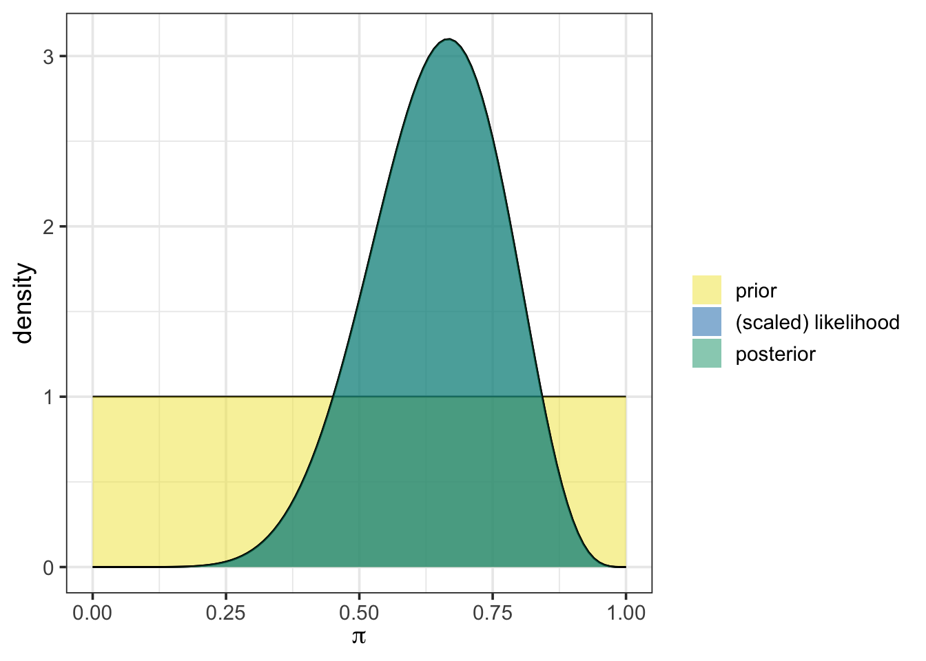
This activity is a context-free scaffold. You’ll almost surely find it to be incomplete, and that’s on purpose! We are designing this series of activities to have a domain-specific context laid over them. Throughout the activity, you’ll see purple text, which is text that should be replaced with context-specific content. A rough draft completed activity is available here, in the chytrid fungus context.
Statistics Goals: The statistics-focused goals of this activity are as follows:
{bayesrules} package to easily update a prior with observed data, obtaining a posterior distribution.Course Objectives: This activity would map to course-level objectives similar to the following. Note that this is not an exhaustive list, nor should it be interpreted that objectives must be phrased identically. This is to give an idea as to the wide variety of contexts this activity might be placed in.
Subject-Specific Objectives: This section is where course-specific objectives relevant to the activity’s context can be detailed. This allows instructors to meet objectives specific to their discipline while incorporating Bayesian thinking.
The following sections provide the statistical and contextual background for this activity.
There are many statistical tools which can be used to investigate population parameters. As we mentioned in our first activity, these tools fall into three broad categories:
This series of activities focuses on Bayesian methods. In this second activity, we engage in extracting and interpreting a credible interval from a posterior distribution. We’ll briefly review how to obtain the posterior distribution from the prior and observed data, but check back on our first activity for full details.
This subsection includes background on the domain-specific context for the activity.
Building on concepts from the first activity, we’ll continue to estimate the [relevant population parameter] by extracting and interpreting a credible interval from the posterior distribution.
In Bayesian inference, a prior distribution represents initial beliefs about a population parameter. This allows for prior knowledge or experiences (and uncertainties) to inform conclusions without solely relying on new data. The posterior distribution is then obtained by updating the prior with observed data by using a version of Bayes’ Rule:
\[\mathbb{P}\left[\text{parameter value} \mid \text{data}\right] = \frac{\mathbb{P}\left[\text{data} \mid \text{parameter value}\right]\cdot \mathbb{P}\left[\text{parameter value}\right]}{\mathbb{P}\left[\text{data}\right]}\]
In Activity 1, we manually updated the prior, applying this relationship step-by-step via code, which provided transparency into the Bayesian updating process.
We’ll start with a reminder of where our pre-reading left off before moving on to learn about convenient functionality, how that functionality can help us obtain credible intervals, and how we can interpret and draw insights from those intervals.
Building on concepts from the first activity, we’ll continue to estimate the [relevant population parameter] by extracting and interpreting a credible interval from the posterior distribution.
In Bayesian inference, a prior distribution represents initial beliefs about a population parameter. This allows for prior knowledge or experiences (and uncertainties) to inform conclusions without solely relying on new data. The posterior distribution is then obtained by updating the prior with observed data by using a version of Bayes’ Rule:
\[\mathbb{P}\left[\text{parameter value} \mid \text{data}\right] = \frac{\mathbb{P}\left[\text{data} \mid \text{parameter value}\right]\cdot \mathbb{P}\left[\text{parameter value}\right]}{\mathbb{P}\left[\text{data}\right]}\]
In Activity 1, we manually updated the prior, applying this relationship step-by-step via code, which provided transparency into the Bayesian updating process.
{bayesrules}We’re having trouble with {rstanarm} in webR and {rstanarm} is a dependency of the {bayesrules} package. Since none of the functions utilized in this activity require {rstanarm}, I’ve saved an R Script with the functions we are using. Run the code cell below to “source” that script.
In this activity, we’ll simplify the process of obtaining our posterior distributions by using functions from the {bayesrules} package. Bayes Rules! An Introduction to Bayesian Modeling, by Johnson, Ott, and Dogucu (Johnson, Ott, and Dogucu 2022) and the corresponding {bayesrules} R package (Dogucu, Johnson, and Ott 2021) provide user-friendly functionality that we’ll take advantage of.
In our first activity, we began with an uninformative prior, represented as a beta distribution with one observed success and one failure, beta(1, 1). We then updated that prior with our initially observed data including eight (8) successes out of twelve (12) observations. Using the plot_beta_binomial() and summarize_beta_binomial() functions from {bayesrules}, we can easily visualize and summarize the prior, likelihood, posterior, and associated statistics.
To use plot_beta_binomial(), we need to specify four arguments:
alpha is the number of previously observed successesbeta is the number of previously observed failuresy is the number of newly observed successful outcomesn is the total number of new observations recordedBelow is an example with our initial beta(1, 1) prior and the first set of new observations we encountered:
plot_beta_binomial(alpha = 1, beta = 1, y = 8, n = 12)
In the plot, the prior distribution appears in yellow, while the posterior is shown in blue-green. Here, our uninformative prior results in the posterior overlapping exactly with the scaled likelihood. This is because of our choice to use the uniform prior.
To obtain summary statistics on the prior and posterior, we use the summarize_beta_binomial() function, which provides key characteristics of each distribution, including the mean, mode, standard deviation, and variance. This function takes the same arguments as plot_beta_binomial().
summarize_beta_binomial(alpha = 1, beta = 1, y = 8, n = 12)| model | alpha | beta | mean | mode | var | sd |
|---|---|---|---|---|---|---|
| prior | 1 | 1 | 0.5000000 | NaN | 0.0833333 | 0.2886751 |
| posterior | 9 | 5 | 0.6428571 | 0.6666667 | 0.0153061 | 0.1237179 |
We’ll quickly revisit the second investigation we made in that initial activity as well. You may remember that we obtained advice from an expert, indicating that we suspect that the population proportion should be near 60%, given prior research results. At that point, we re-evaluated our choice of prior distribution to reflect this. We chose a weak prior, which was still a beta distribution but with 6 previously observed successes and 4 previously observed failures. Such a prior is weak because it assumes information from very few previous observations.
Let’s plot that prior, along with the scaled likelihood and posterior distribution using plot_beta_binomial(). We’ll also obtain the numerical summaries for the prior and posterior distributions while we are at it.
plot_beta_binomial(alpha = 6, beta = 4, y = 8, n = 12)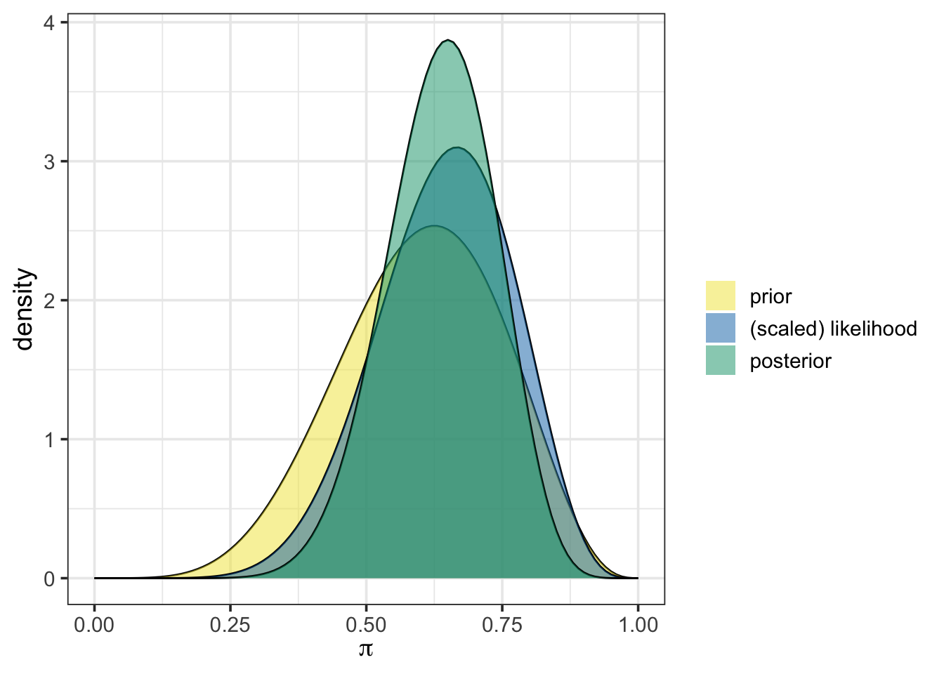
summarize_beta_binomial(alpha = 6, beta = 4, y = 8, n = 12)| model | alpha | beta | mean | mode | var | sd |
|---|---|---|---|---|---|---|
| prior | 6 | 4 | 0.6000000 | 0.625 | 0.0218182 | 0.1477098 |
| posterior | 14 | 8 | 0.6363636 | 0.650 | 0.0100611 | 0.1003050 |
From the output above, we can see that the prior, the scaled likelihood, and the posterior are all distinct. The prior and the likelihood of our observed data act together to arrive at the posterior distribution. Again, the use of plot_beta_binomial() simplifies our job by performing the Bayesian update behind the scenes.
While we are transitioning to the more “black box” functionality in this activity (and you’ll continue with similar functionality in the remaining activities, too), the foundation you built in engaging with the first activity should give you some intuition around what functions like plot_beta_binomial() and summarize_beta_binomial() are doing when they are run.
Take this opportunity to discuss what is happening “behind the scenes” when the plot_beta_binomial() function is run.
Through the main section of this activity, you’ll explore the use of credible intervals (CIs), the Bayesian analog to the Frequentist’s confidence interval. A key advantage of credible intervals is that they offer a much more intuitive interpretation. For example, with a 95% credible interval, we claim there is a 95% probability that the population parameter lies within the interval bounds.
Before we get into CIs, let’s get ourselves back to where we were at the end of the last activity. As you might remember, we obtained the following data.
As a reminder, we can set up this code chunk so that the data is
simulated, as in the code chunk below.
read in from a location on the web (for example, a GitHub repository). This could be data from a study, a publication, your own research, etc.
collected in class and manually input into the status column of the tibble below.
The code below will be replaced based on the choice made above.
Use the plot_beta_binomial() and summarize_beta_binomial() functions in the code cell below to update your weakly informative beta(6, 4) prior with these 157 observations including 102 positive outcomes.
When observing the results from these two functions, consider the following questions.
Notice that this new data updates our prior beliefs about our population parameter. The posterior distribution now represents our updated “world-view” after seeing new evidence.
If you’ve taken a traditional (Frequentist) statistics course, you might be familiar with confidence intervals. These intervals aim to capture a population parameter with a prescribed level of certainty. In practice, however, interpreting these intervals can be tricky. Confidence intervals are based on a hypothetical scenario in which we take many random samples and build intervals from each; the expectation is that, over many intervals, a certain proportion (like 95% for a 95% confidence interval) would contain the true parameter.
In Bayesian inference, credible intervals offer a simpler, probabilistic interpretation. A 90% credible interval extends from the 5th percentile to the 95th percentile of the posterior distribution. This means there’s a 90% probability that the population parameter falls within these bounds, based on the prior assumption and the observed data — no hypothetical repetitions required.
In this section of our activity, we’ll compute and interpret credible intervals. To do so, we’ll need a bit of information about the qbeta() function, which calculates “quantiles” from a beta distribution. To use qbeta(), we input the proportion of observations to the left of the desired quantile, along with the \(\alpha\) and \(\beta\) parameters defining the distribution. This returns the cutoff value at the desired quantile.
For example, we calculate the \(5^{\text{th}}\) and \(95^{\text{th}}\) percentiles from our weakly informative beta(6, 4) prior, giving us a 90% credible interval below.
lower_bound <- qbeta(0.05, 6, 4)
upper_bound <- qbeta(0.95, 6, 4)

lower_bound
[1] 0.3449414upper_bound[1] 0.8312495So, based on our prior, we have a 90% probability that the population parameter falls between about 34.5% and about 83.1%. Note that we could have also calculated both of these bounds at once using qbeta(c(0.05, 0.95), 6, 4).
We can also visualize this confidence interval by using the plot_beta_ci() function, which takes \(\alpha\), \(\beta\) and the desired level of coverage as arguments.
plot_beta_ci(6, 4, 0.90)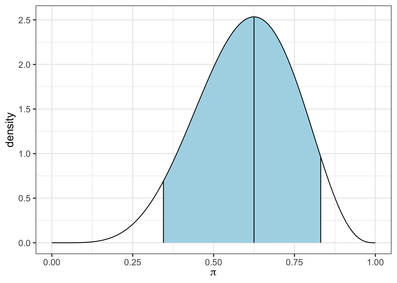
Now, use the updated data (the 102 positive outcomes from the 157 observations) and your results from summarize_beta_binomial(), along with the qbeta() function to extract a new 90% credible interval for the population proportion from your posterior distribution. Use plot_beta_ci() to plot the credible interval as well.
Now calculate a 95% credible interval for the population proportion.
In this notebook we,
Reflect on where you could apply this new knowledge of credible intervals. Consider examples from: