This activity is a context-free scaffold. You’ll almost surely find it to be incomplete, and that’s on purpose! We are designing this series of activities to have a domain-specific context laid over them. Throughout the activity, you’ll see purple text, which is text that should be replaced with context-specific content. A rough draft completed activity is available here.
Goals and Objectives
Statistics Goals: The statistics-focused goals of this activity are as follows:
Introduce students to the foundational aspects of Bayesian Inference as an alternative to Frequentist methods.
In particular, students discover and examine what a parameter distribution is.
Students discover the notion and impact of the choice of a prior distribution on the resulting posterior parameter distribution.
Students discover the impact of amount of data on the resulting posterior parameter distribution.
Students experiment with how the choice of prior parameter distribution and data interact to influence the resulting posterior parameter distribution.
Course Objectives: This activity would map to course-level objectives similar to the following. Note that this is not an exhaustive list, nor should it be interpreted that objectives must be phrased identically. This is to give an idea as to the wide variety of contexts this activity might be placed in.
Students will evaluate a research question using appropriate statistical techniques
Students will correctly identify the type of data they are working with
Students will evaluate literature and/or prior research to generate hypotheses for a research question
Students will learn about different statistical models and approaches
Students will interpret coefficients from a statistical model
Students will evaluate the underlying assumptions of a statistical approach
Students will consider the ethical implications of statistical approaches
Students will gather data using methodologies appropriate to the context
Subject-Area Objectives: This section will be utilized to identify objectives/outcomes specific to the course/subject to which the activity context is linked. This allows adopters to cover objectives associated with their course while embedding Bayesian thinking.
Background Information
The following subsections outline the background information for this activity from both a statistics and domain-specific lens.
Data Analysis and Bayesian Thinking
There are many statistical tools which can be used to investigate population parameters. Broadly speaking, these tools fall into three categories:
Classical/Frequentist methods
Simulation-based methods
Bayesian methods
Perhaps you’ve encountered frequentist methods previously. These methods depend on distribution assumptions and the Central Limit Theorem. In this notebook, we’ll introduce Bayesian methods. In particular, you’ll explore how your prior belief (controlled via your choice of prior distribution) and the strength of your observed data work together to produce updated beliefs (a posterior distribution).
In Bayesian inference, we approach our tasks with some prior belief about the value of our population parameter. This is natural, because it matches our lived experience as humans. We use that prior belief, in conjunction with our data, to produce an updated version of our beliefs. Again, likely matching our individual approaches to interacting with the world we live in.
In this interactive notebook, you’ll see the foundations of the Bayesian approach to inference on a [choose the parameter relevant to the context: (population proportion / population mean)] in action. You’ll explore how your prior belief (controlled via your choice of prior distribution) and the strength of your observed data work together to produce updated beliefs.
About the Context
This subsection includes background on the domain-specific context for the activity.
Purpose
Let’s try to estimate the [population parameter in context].
Prior Assumptions
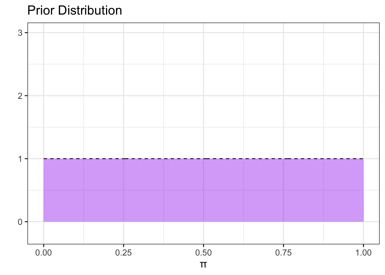
A paragraph indicating the assumptions we might come with if we had no prior expectations about our parameter. The end result here should be that we land on a uniform prior. The code chunk below sets up an uninformative uniform prior for [the population proportion being estimated].
Internal Question (Delete Once Resolved)
Is it necessary that we begin from a uniform prior? I think, for illustration purposes, it is helpful.
alpha <-1beta <-1#Fewer points results in more jagged picturesgrid_pts <-500#Create prior distribution my_dists_prop <-tibble(pi =seq(0, 1, length.out = grid_pts), #possible proportion valuesprior_prob =dbeta(pi, alpha, beta) #prior probability)#Plot prior distributionmy_dists_prop %>%ggplot() +geom_area(aes(x = pi, y = prior_prob), fill ="purple", alpha =0.4) +geom_line(aes(x = pi, y = prior_prob),linetype ="dashed") +labs(title ="Prior Distribution",x ="π",y ="" ) +ylim(c(-0.2, 3))
Shape of Prior
The Beta-distribution we use here is commonly used with binomial data. It is determined by two shape parameters alpha (\(\alpha\)) and beta (\(\beta\)). We can think of \(\alpha\) as the number of previously observed successes and \(\beta\) as the number of previously observed failures. Choosing \(\alpha = 1\) and \(\beta = 1\), results in a prior that allows for both successes and failures (\(\pi \neq 0\) and \(\pi \neq 1\)) but which has no other certainty about the true value of \(\pi\).
Observed Data
In this section, we either generate, read, or collect data which we’ll use to update our chosen prior distribution. The code chunk below is a placeholder which simulates new observed data from our population. As mentioned, there are several options for how this section on Observed Data can be treated.
Observed data can be simulated, as in the code chunk below.
Observed data can be read in from a location on the web (for example, a GitHub repository). This could be data from a study, a publication, your own research, etc.
Observed data can be collected in class and manually input into the status column of the tibble below.
nobs <-12set.seed(071524)my_data <-tibble(obs_id =1:nobs,status =sample(c("yes", "no"), size = nobs,prob =c(0.7, 0.3), replace =TRUE))num_yes <- my_data %>%filter(status =="yes") %>%nrow()print(paste0("Of the ", nobs," observations, the number of positive responses was ", num_yes,"."))
[1] "Of the 12 observations, the number of positive responses was 8."
Obtaining the Posterior
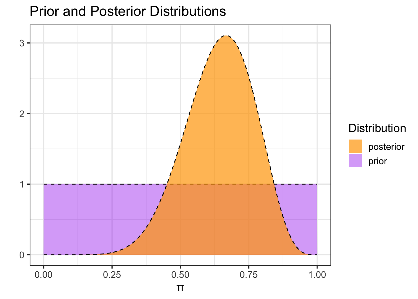
Now we’ll use our data to update the prior distribution and obtain the posterior distribution for our population proportion. We obtain the posterior distribution by multiplying the prior by the likelihood function and then dividing by a normalizing factor to ensure that the result is a probability density (that is, the total probability is 1). The likelihood measures the probability of observing our data at each possible value of the population proportion.
The code chunk below constructs the posterior distribution according to the Bayesian-Updating procedure above.
#Construct the posteriormy_dists_prop <- my_dists_prop %>%mutate(#Compute likelihood using binomial distributionlikelihood =choose(nobs, num_yes)*pi^(num_yes)*(1- pi)^(nobs - num_yes), #Compute posterior as likelihood*priorpost_prob = likelihood*prior_prob,#Normalize posteriorpost_prob_normalized = post_prob/(sum(post_prob)*1/grid_pts))#Plot prior and posteriormy_dists_prop %>%ggplot() +geom_area(aes(x = pi, y = prior_prob, fill ="prior"), alpha =0.4) +geom_line(aes(x = pi, y = prior_prob),linetype ="dashed") +geom_area(aes(x =pi, y = post_prob_normalized, fill ="posterior"), alpha =0.7) +geom_line(aes(x = pi, y = post_prob_normalized),linetype ="dashed") +labs(title ="Prior and Posterior Distributions",x ="π",y ="",fill ="Distribution" ) +scale_fill_manual(values =c("prior"="purple", "posterior"="orange"))
Notice that, after seeing the data, our posterior estimate for the proportion of [insert context here] has been updated. [We’ll summarize what we are seeing here, or even better…ask the students to do that via a question in this location.]
Investigating Further
Now that you’ve seen one Bayesian analysis to estimate [insert population parameter here], let’s reproduce the analysis and explore the impact of (i) choice of prior, (ii) strength of data, and (iii) the combination of data and prior on the resulting posterior.
In this section, you’ll have an opportunity to reproduce the analysis above, but with a different choice of prior distribution on \(\pi\).
Update from an Expert
This box will provide students with an update, providing them with valuable information they can use to choose a more informative prior.
Recall that, in the Beta distribution, the two parameters alpha (\(\alpha\)) and beta (\(\beta\)) can be thought of as the number of prior successes and prior failures, respectively. Update the code chunk below to choose an alpha and beta that reflects the new information provided in the box above.
Once you’ve made the update, run the code to construct and visualize the prior.
Reflection Question
How does this prior compare to our original prior? Use your understanding of alpha and beta to justify what you are seeing.
Now that you’ve built the new prior, run the code chunk below to recognize your new data. Again, for the code chunk, we have the following options.
Observed data can be simulated, as in the code chunk below.
Observed data can be read in from a location on the web (for example, a GitHub repository). This could be data from a study, a publication, your own research, etc.
Observed data can be collected in class and manually input into the status column of the tibble below.
Now run the code chunk below to use the observed data to calculate and plot the updated posterior.
Reflection Question
How does this new posterior compare to the original posterior distribution we estimated? What effect has our choice of stronger prior had on the range of proportions you think our population parameter may live within? Does this result match your expectations?
In this section, you’ll have an opportunity to reproduce our original analysis using the flat prior, but with a different data source for updating. In particular, you’ll explore the impact that the number of collected observations can have on the resulting posterior distribution.
Update from an Expert
This box will provide students with an update, providing them with a description or location of newly collected data. The new data source should have many more observations than the original data source. For example, the original data source could just have been a small random sample from an existing, larger data source.
A Question about Activity Design
The correct thing to do here would be to use this new data to update our previous posterior distribution. This adds more complexity/intricacy to the activity though. What is the tradeoff between explaining a second update to the posterior versus going back to the original prior and updating it with all of the observed data? With the beta-binomial the results will be the same but I don’t want to build bad habits/poor understanding by taking a simplistic approach here.
Possible paths forward:
Address that the correct thing to do would be to update the posterior with the new data, but leave the simplified approach in here and mention that the results are identical in this case.
Drawbacks: This does not illustrate how learners should do Bayesian inference in the future.
Explain that statistical inference can be an iterative process in which we continue updating our understanding as new data is collected. Replace the prior with the posterior and use the data to update again.
Drawbacks: This might mask the takeaway that we are trying to lead students to – lots of data can have great influence in updating to the posterior. Perhaps we can accomplish both goals if the initial set of observations is small enough.
Laura’s response: I would err on the side of good practice, even if it complicates things. Alternatively, what if we had a side-by-side: update with little data, update with lots of data - see difference? Or would that be massively confusing?
The code chunk below is set to create a weakly informative prior that assumes the additional information we received from the previous scenario, but from a small sample. For now we set a prior from 10 observations with 6 positive results, for illustration purposes.
Now that we have this prior, run the code cell below to generate the observed data. Don’t make any changes to the code just yet. As a reminder, we can set up this code chunk so that the data is
simulated, as in the code chunk below.
read in from a location on the web (for example, a GitHub repository). This could be data from a study, a publication, your own research, etc.
collected in class and manually input into the status column of the tibble below.
This is an unlikely choice due to the relatively small sample size and time required to input data. This method could be accommodated if data is collected via a digital form and then read from a spreadsheet (ie. Google Forms/Sheets).
The code below will be replaced based on the choice made above.
Now run the code chunk below to use the observed data to calculate and plot the updated posterior.
Reflection Question
How does this new posterior compare to the original posterior distribution we estimated? What effect has our larger collection of observations (larger sample size) had on the range of proportions you think our population parameter may live within? Does this result match your expectations?
Now that you’ve seen how different priors and data (separately) result in different inferences, return to the previous section and examine how stronger priors (for example, alpha = 600 and beta = 400) interact with our data to form the resulting posterior.
Reflection Question
What conclusions can you draw about whether the prior or the observed data has greater influence over the resulting posterior?