From the Prior to the Posterior

(Biology; Chytrid Fungus in Frogs)

Authors

Affiliations

Adam Gilbert

Southern New Hampshire University

Katie Duryea

Southern New Hampshire University

Laura Lambert

James Madison University

Sample Activity 1 (Biology Context)

This activity is a sample of our first activity (From the Prior to the Posterior) with a biology context laid over the framework. This sample has been constructed with coauthor Dr. Katie Duryea, a member of the Biology faculty at Southern New Hampshire University. This sample activity provides an example of what versions of this activity from other domains/contexts may look like.

Goals and Objectives

Goals: The goals of this activity are as follows:

• Show students an alternative to the Frequentist approach to capturing a population parameter.
• Students discover the impact of choice of prior on their plausible range.
• Students discover the impact of amount of data on their plausible range.

Course Objectives: This activity would map to course-level objectives similar to the following. Note that this is not an exhaustive list, nor should it be interpreted that objectives must be phrased identically. This is to give an idea as to the wide variety of contexts this activity might be placed in.

• Students will evaluate a research question using appropriate statistical techniques
• Students will correctly identify the type of data they are working with
• Students will evaluate literature and/or prior research to generate hypotheses for a research question
• Students will learn about different statistical models and approaches
• Students will interpret coefficients from a statistical model
• Students will evaluate the underlying assumptions of a statistical approach
• Students will examine the ecological impact of different pathogens, both native and introduced
• Students will consider the ethical implications of statistical approaches
• Students will gather data using methodologies appropriate to the context

Biology Objectives: I’ll work with Katie to add drafts of these objectives.

Background Information

The following subsections outline the background information for this activity from both a statistics and domain-specific lens.

Data Analysis and Bayesian Thinking

There are many statistical tools which can be used to test hypotheses about population parameters. Broadly speaking, these tools fall into three categories:

• Classical/Frequentist methods
• Simulation-based methods
• Bayesian methods

Perhaps you’ve encountered frequentist methods previously. These methods depend on distribution assumptions and the Central Limit Theorem. In this notebook, we’ll introduce Bayesian methods. In particular, you’ll explore how your prior belief (controlled via your choice of prior distribution) and the strength of your observed data work together to produce updated beliefs (a posterior distribution).

In Bayesian inference, we approach our tasks with some prior belief about the value of our population parameter. This is natural, because it matches our lived experience as humans. We use that prior belief, in conjunction with our data, to produce an updated version of our beliefs. Again, likely matching our individual approaches to interacting with the world we live in.

In this interactive notebook, you’ll see the foundations of the Bayesian approach to inference on a [choose the parameter relevant to the context: (population proportion / population mean)] in action. You’ll explore how your prior belief (controlled via your choice of prior distribution) and the strength of your observed data work together to produce updated beliefs.

About Chytrid

Chytrid fungus is an infectious fungal disease that can be fatal to amphibians and has caused some species to become extinct. Check out this video from Chris Egnoto to learn more about this threat to amphibian life.

Purpose

Let’s try to estimate the proportion of frogs in southern New Hampshire which are impacted by chytrid fungus.

Prior Assumptions

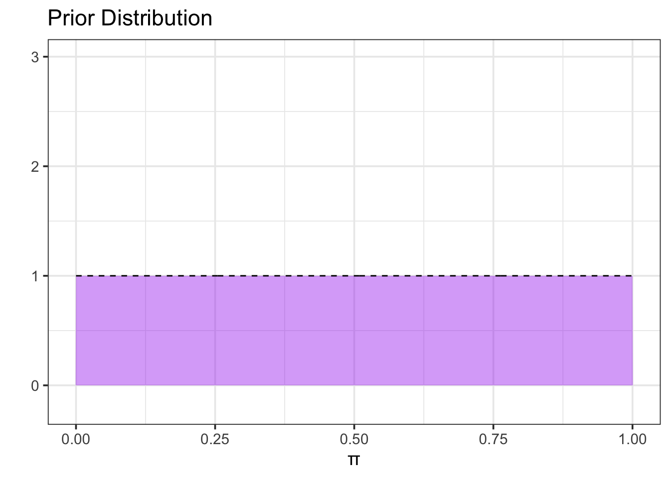
Perhaps today is our first time learning about chytrid fungus and frogs. We may have no expectation about what our population proportion (\(\pi\)) might be. In the Frequentist approach, we would let the data completely determine the inference we make about the proportion. In Bayesian inference, we take a different approach and assign a prior distribution over the population proportion we are looking for. Since today is the first we’ve heard of Chytrid, let’s set up a prior that indicates nearly all values of \(\pi\) are equally likely.

alpha <- 1
beta <- 1
#Fewer points results in more jagged pictures
grid_pts <- 500

#Create prior distribution 
my_dists <- tibble(
  pi = seq(0, 1, length.out = grid_pts), #possible proportion values
  prior_prob = dbeta(pi, alpha, beta) #prior probability
)

#Plot prior distribution
my_dists %>%
  ggplot() + 
  geom_area(aes(x = pi, y = prior_prob), 
            fill = "purple", alpha = 0.4) + 
  geom_line(aes(x = pi, y = prior_prob),
            linetype = "dashed") + 
  labs(
    title = "Prior Distribution",
    x = "π",
    y = ""
  ) + 
  ylim(c(-0.2, 3))

Shape of Prior

The Beta-distribution we use here is commonly used with binomial data. It is determined by two shape parameters alpha (\(\alpha\)) and beta (\(\beta\)). We can think of \(\alpha\) as the number of previously observed successes and \(\beta\) as the number of previously observed failures. Choosing \(\alpha = 1\) and \(\beta = 1\), results in a prior that allows for both successes and failures (\(\pi \neq 0\) and \(\pi \neq 1\)) but which has no other certainty about the true value of \(\pi\).

Observed Data

In the actual activity, we’ll read in real data below. For now, let’s generate some fake data.

num_frogs <- 12
set.seed(071524)
my_data <- tibble(
  frog_number = 1:num_frogs,
  status = sample(c("positive", "negative"), 
                  size = num_frogs,
                  prob = c(0.7, 0.3), 
                  replace = TRUE)
)

num_pos <- my_data %>%
  filter(status == "positive") %>%
  nrow()

print(paste0("Of the ", num_frogs, 
             " frogs observed, the number positive for Chytrid fungus was ", 
             num_pos, "."))

[1] "Of the 12 frogs observed, the number positive for Chytrid fungus was 8."

Obtaining the Posterior

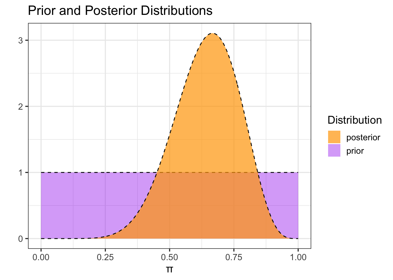
Now we’ll use our data to update the prior distribution and obtain the posterior distribution for our population proportion. We obtain the posterior distribution by multiplying the prior by the likelihood function and then dividing by a normalizing factor to ensure that the result is a probability density (that is, the total probability is 1). The likelihood measures the probability of observing our data at each possible value of the population proportion.

\[\underbrace{\mathbb{P}\left[\text{proportion} | \text{data}\right]}_{\text{posterior}} = \frac{\overbrace{\mathbb{P}\left[\text{data} | \text{proportion}\right]}^{\text{likelihood}}\cdot \overbrace{\mathbb{P}\left[\text{proportion}\right]}^{\text{prior}}}{\underbrace{\mathbb{P}\left[\text{data}\right]}_{\text{normalizing factor}}}\]

#Construct the posterior
my_dists <- my_dists %>%
  mutate(
    #Compute likelihood using binomial distribution
    likelihood = choose(num_frogs, num_pos)*pi^num_pos*(1 - pi)^(num_frogs - num_pos), 
    #Compute posterior as likelihood*prior
    post_prob = likelihood*prior_prob,
    #Normalize posterior
    post_prob_normalized = post_prob/(sum(post_prob)*1/grid_pts))

#Plot prior and posterior
my_dists %>%
  ggplot() + 
  geom_area(aes(x = pi, y = prior_prob, fill = "prior"), 
            alpha = 0.4) + 
  geom_line(aes(x = pi, y = prior_prob),
            linetype = "dashed") + 
  geom_area(aes(x = pi, y = post_prob_normalized, fill = "posterior"), 
            alpha = 0.7) + 
  geom_line(aes(x = pi, y = post_prob_normalized),
            linetype = "dashed") +
  labs(
    title = "Prior and Posterior Distributions",
    x = "π",
    y = "",
    fill = "Distribution"
  ) +
  scale_fill_manual(values = c("prior" = "purple", "posterior" = "orange"))

Notice that, after seeing the data, our posterior estimate for the proportion of frogs impacted by Chytrid has been updated. It looks very unlikely that \(\pi\) is less than 0.25 (those population proportions seem incompatible with our observed data), and the most likely proportions are between 0.5 and 0.8.

Investigating Further

Now that you’ve seen one Bayesian analysis to estimate the proportion of frogs impacted by Chytrid, let’s reproduce the analysis and explore the impact of (i) choice of prior, (ii) strength of data, and (iii) the combination of data and prior.

Influence of the Prior

In this section, you’ll have an opportunity to reproduce the analysis above, but with a different choice of prior distribution on \(\pi\).

From Dr. Duryea

[This is a placeholder for now…] In her research, Dr. Duryea has noted that approximately 60% of frogs are impacted by Chytrid.

Recall that, in the Beta distribution, the two parameters alpha (\(\alpha\)) and beta (\(\beta\)) can be thought of as the number of prior successes and prior failures, respectively. Update the code chunk below to choose an alpha and beta that will result in the 60% estimate observed by Dr. Duryea in her research. Run the code to construct and visualize your prior.

Reflection Question

How does this prior compare to our original prior? Use your understanding of alpha and beta to justify what you are seeing.

Now that you’ve built this new prior, run the code cell below to generate the observed data. Don’t make any changes to the code just yet (Note: I don’t think I want this here, but keep it for now).

Now run the code chunk below to use the observed data to calculate and plot the updated posterior.

Reflection Question

How does this new posterior compare to the original posterior distribution we estimated? What effect has our choice of stronger prior had on the range of proportions you think our population parameter may live within? Does this result match your expectations?

Influence of Data

In this section you’ll have an opportunity to reproduce the analysis above, but with different data sources for updating. In particular, you’ll explore the impact that the number of observations can have on the posterior distribution.

From Dr. Duryea

[This is a placeholder for now…] Dr. Duryea’s students have finished processing their most recent collection of samples. She has provided us with a larger collection of observed data. Let’s see the impact that this larger data set has on updating the prior distribution.

The code chunk below is set to create a weakly informative prior that assumes a population proportion of chytrid fungus infection of 60%, backed by a total of 10 observations. Run the code to construct and visualize this prior.

Now that we have this prior, run the code cell below to generate the observed data. Don’t make any changes to the code just yet (Note: I don’t think I want this here, but keep it for now).

Now run the code chunk below to use the observed data to calculate and plot the updated posterior.

Reflection Question

How does this new posterior compare to the original posterior distribution we estimated? What effect has our larger collection of observations (larger sample size) had on the range of proportions you think our population parameter may live within? Does this result match your expectations?

Combined Influence

Now that you’ve seen how different priors and different data (separately) result in different inferences, return to the previous section and examine how stronger priors (for example alpha = 600 and beta = 400) interact with our data to influence our inference.

Reflection Question

What conclusions can you draw about whether the prior or the observed data has greater influence over the resulting posterior?