Simple Linear Regression: Construction, Assessment, and Interpretation

Dr. Gilbert

October 1, 2024

The Highlights

• What is Simple Linear Regression?

• What are we assuming?

• Global tests for model utility and the individual term-based test.

• Further model assessment

  • Validation metrics
  • Residual analysis

• Model interpretation

• Predictions

What is Simple Linear Regression?

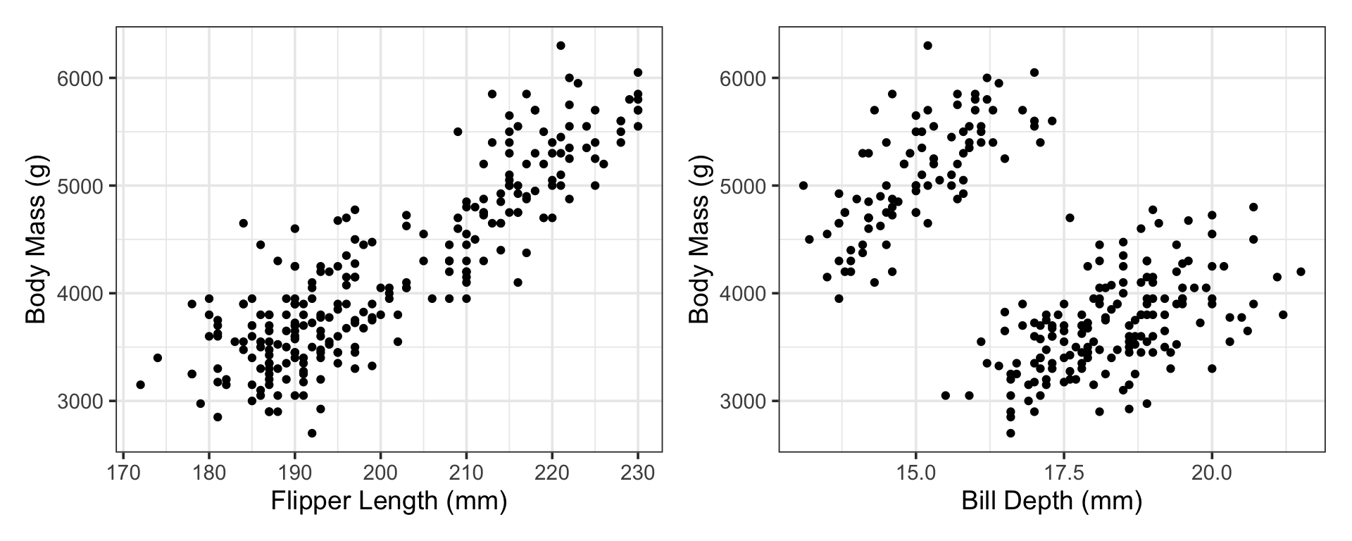
Question 1 (Inferential): What, if anything, is the relationship between penguin flipper length and body mass?

Question 1 (Predictive): Can we use penguin flipper length to predict body mass?

Question 2 (Inferential): What, if anything, is the relationship between penguin bill depth and body mass?

Question 2 (Predictive): Can we use penguin bill depth to predict body mass?

What is Simple Linear Regression?

Each of these questions can be answered by the construction and analysis of a model.

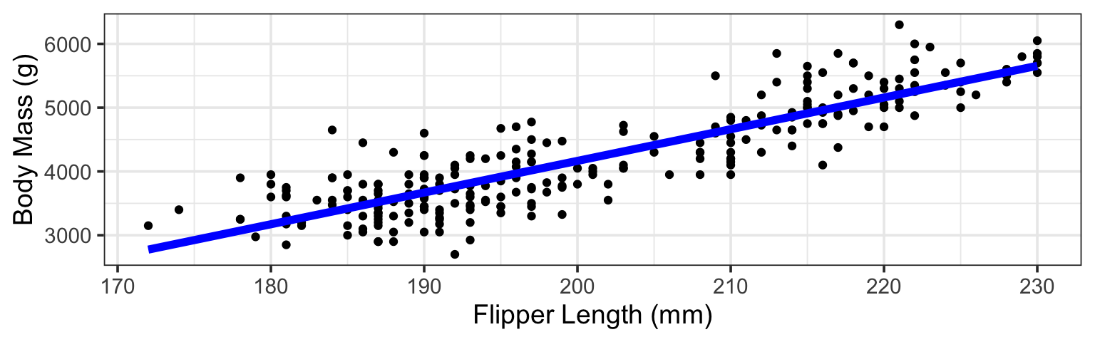
Simple linear regression predicts a response as a linear function of a single predictor variable.

\[\mathbb{E}\left[\text{body mass}\right] = \beta_0 + \beta_1\cdot \left(\text{flipper length}\right)\\ \textbf{or}\\ \mathbb{E}\left[\text{body mass}\right] = \beta_0 + \beta_1\cdot \left(\text{bill depth}\right)\]

What is Simple Linear Regression?

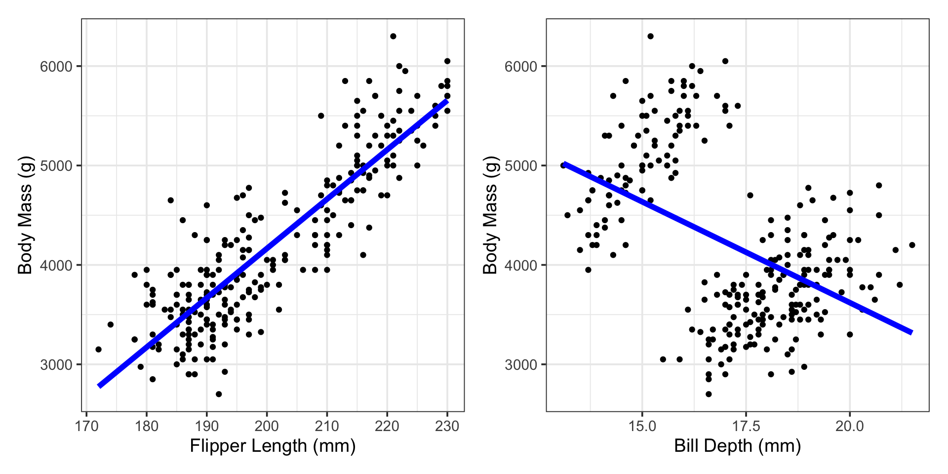
\[\mathbb{E}\left[\text{body mass}\right] = -5769 + 49.7\left(\text{flipper length}\right)\\ \textbf{or}\\ \mathbb{E}\left[\text{body mass}\right] = 7697 - 203\left(\text{bill depth}\right)\]

Let’s Play Along

\(\bigstar\) As usual, I recommend that you play along during our discussion! \(\bigstar\)

1. Open RStudio
2. Verify that you are working within your MAT300 project space
3. Open your most recent notebook – the one where you built a simple linear regressor to predict the rental price of an Air BnB
4. Run all of the code chunks in that notebook
5. Describe the inferential and predictive questions you implicitly asked in pursuing the construction of our simple linear regression models from the end of our last class meeting

What Are We Assuming?

\[\mathbb{E}\left[\text{body mass}\right] = \beta_0 + \beta_1\cdot\left(\text{flipper length}\right)\]

Pre-Modeling Assumptions: Penguin body mass is associated with penguin flipper length in a linear manner, independent of all other possible features.

Post-Modeling Assumptions: The following assumptions are made about model errors (residuals), to ensure that using and interpreting the model is appropriate.

• Residuals are normally distributed
• Residuals are independent of one another, the predictor, predictions, and the response
• The standard deviation of residuals is constant with respect to the predictor, predictions, and the response

Global and Term-Based Model Assessments

Global Test for Model Utility: \(\begin{array}{lcl} H_0 & : & \beta_1 = 0\\ H_a & : &\beta_1 \neq 0\end{array}\)

r.squared	adj.r.squared	sigma	statistic	p.value	df	logLik	AIC	BIC	deviance	df.residual	nobs
0.7646157	0.763689	398.8774	825.0863	0	1	-1895.34	3796.68	3807.315	40412211	254	256

Individual Term-Based Assessment: \(\begin{array}{lcl} H_0 & : & \beta_1 = 0\\ H_a & : &\beta_1 \neq 0\end{array}\)

term	estimate	std.error	statistic	p.value
(Intercept)	-5768.75714	348.042020	-16.57489	0
flipper_length_mm	49.67168	1.729255	28.72431	0

For Simple Linear Regression, the Global Test for Model Utility and the Term-based test have the same hypotheses and will have the same \(p\)-value. They are the same test here!

Additional [Training] Performance Metrics

lin_reg_flip_fit %>%
  glance()

metric	value
r.squared	0.7646157
adj.r.squared	0.7636890
sigma	398.8774178
statistic	825.0862647
p.value	0.0000000
df	1.0000000
logLik	-1895.3397992
AIC	3796.6795984
BIC	3807.3151307
deviance	40412211.3860991
df.residual	254.0000000
nobs	256.0000000

• \(R^2_{\text{adj}} \approx 76.4\%\), so approximately 76.4% of variation in penguin body mass is explained by variation in flipper length.

• Training RMSE (sigma) is about 398.88, so we expect our model to predict penguin body mass to within \(\pm 2\cdot\left(398.88\right) \approx \pm 797.76\) grams.

  • Note that this estimate is likely too optimistic.

Accessing and Interpreting Global and Term-Based Performance Metrics

\(\bigstar\) Let’s try it! \(\bigstar\)

1. Obtain the global model performance metrics for your model

   • Hint. You’ll need the glance() function for this

2. Analyse and interpret the result

3. Obtain the individual term-based model assessment metrics

   • Hint. You’ll need to use extract_fit_engine() here

4. Analyse and interpret the result

Additional [Validation] Performance Metrics

my_metrics <- metric_set(
  rmse, rsq
  )

lin_reg_flip_fit %>%
  augment(penguins_test) %>%
  my_metrics(.pred, 
             body_mass_g)

.metric	.estimate
rmse	380.8203026
rsq	0.7405649

• \(R^2 \approx 74.1\%\), so approximately 74.1% of variation in penguin body mass is explained by variation in flipper length, when taking away the training data advantage.

• Test RMSE is about 380.82, so we expect our model to predict penguin body mass to within \(\pm 2\cdot\left(380.82\right) \approx \pm 761.64\) grams.

• The test \(R^2\) value is slightly worse than the corresponding training metric, while the test RMSE is an improvement over the training RMSE.

  • Generally, we should expect slightly worse performance on the test data than on training data.

Performance Metrics on Validation Data

\(\bigstar\) Let’s try it! \(\bigstar\)

1. Use the code from the previous slide to obtain model performance metrics measured on the validation data (the test set)
2. How do the training and validation metrics compare with one another?

Residual Analysis

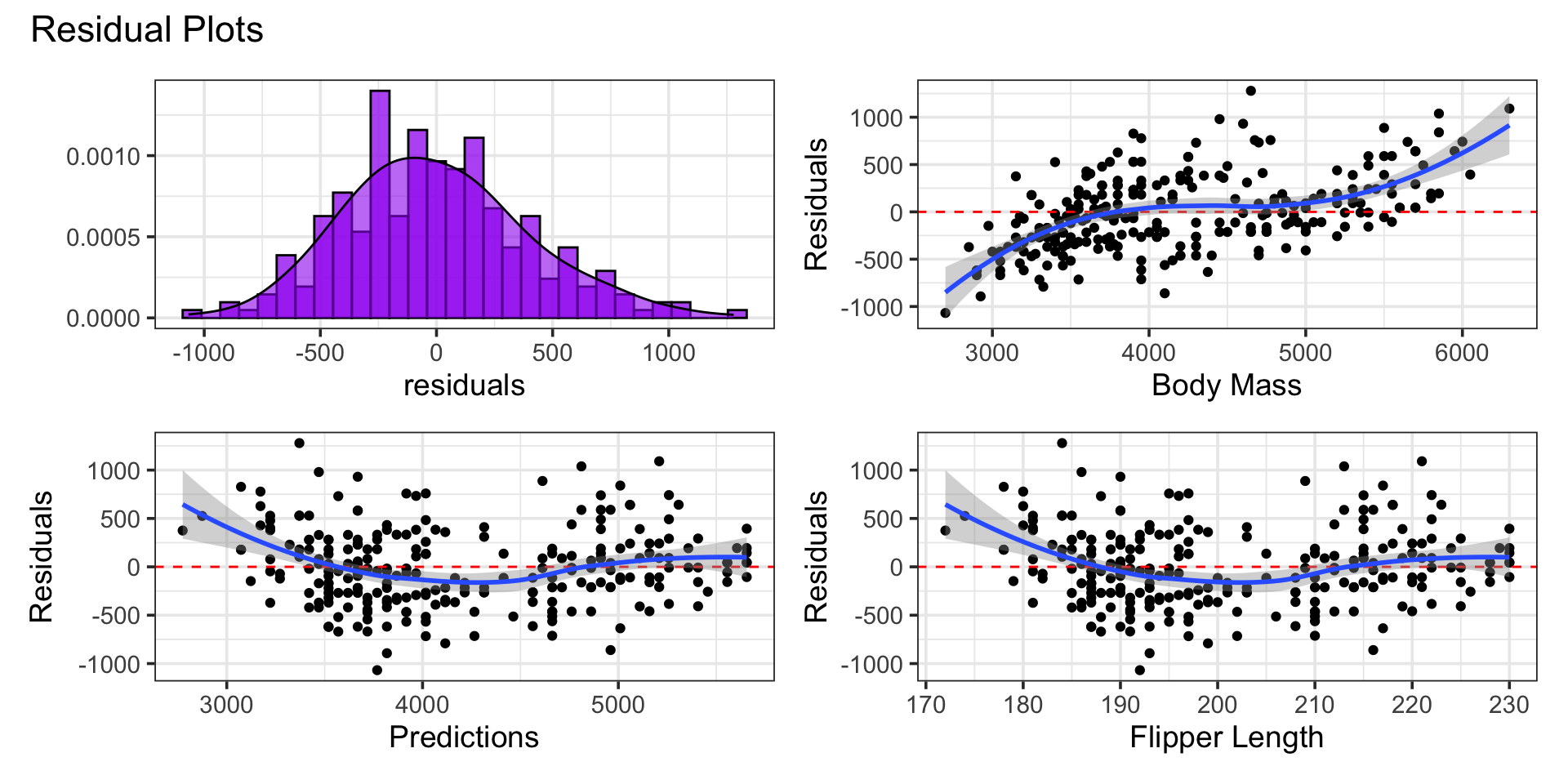
The residuals look approximately normal – with some right skew. There does seem to be an association between the residuals and response, predictions, and flipper length though.

Patterns in residual plots indicate that we could make a better model.

Conducting a Residual Analysis

\(\bigstar\) Let’s try it! \(\bigstar\)

1. Attach your model’s predictions to your training data

2. Compute a residuals (prediction errors) column

3. Visualize the distribution of residuals

4. Create a plot between residuals and the response

5. Create a plot between residuals and the predictions

6. Create a plot between the residuals and the predictor

7. Interpret the plots you’ve constructed

   • What do you notice about the plots between resduals and predictor and residuals and predictions? Why might this be?

Model Interpretations

term	estimate	std.error	statistic	p.value
(Intercept)	-5768.75714	348.042020	-16.57489	0
flipper_length_mm	49.67168	1.729255	28.72431	0

\[\mathbb{E}\left[\text{body mass}\right] = -5768.76 + 49.67\cdot\left(\text{flipper length}\right)\]

Interpretations:

• (Intercept) We expect a penguin whose flipper length measures 0mm to have a mass of about -5768.76g

  • Note that this is not reasonable, and our model doesn’t support this interpretation since our shortest observed flipper length was 172mm.
  • We could force the intercept to be 0, but we would observe worse fit.

• (Flipper Length) We expect a 1mm increase in flipper length to be associated with about a 49.67g increase in penguin body mass, on average.

Model Interpretations

\(\bigstar\) Let’s try it! \(\bigstar\)

1. Extract your model fit

2. Provide interpretations of the model coefficients

   • Is an interpretation of the intercept meaningful for your model?

3. Include your discussions in your Quarto Notebook

Using the Model to Make Predictions

Consider the following questions:

1. What is the body mass of a penguin whose flipper length is 212mm?
2. What is the average body mass of all penguins whose flipper lengths are 212mm?

The first question is asking about the mass of a single penguin, while the second question is asking about the average mass over all penguins with a particular characteristic.

There is more uncertainty associated with trying to answer the first question.

Our model predicts

\[\begin{align} \mathbb{E}\left[\text{body mass}\right] &= -5768.76 + 49.67\left(212\right)\\ &= 4761.28\text{g} \end{align}\]

as the answer to both – we have 0% confidence in this!

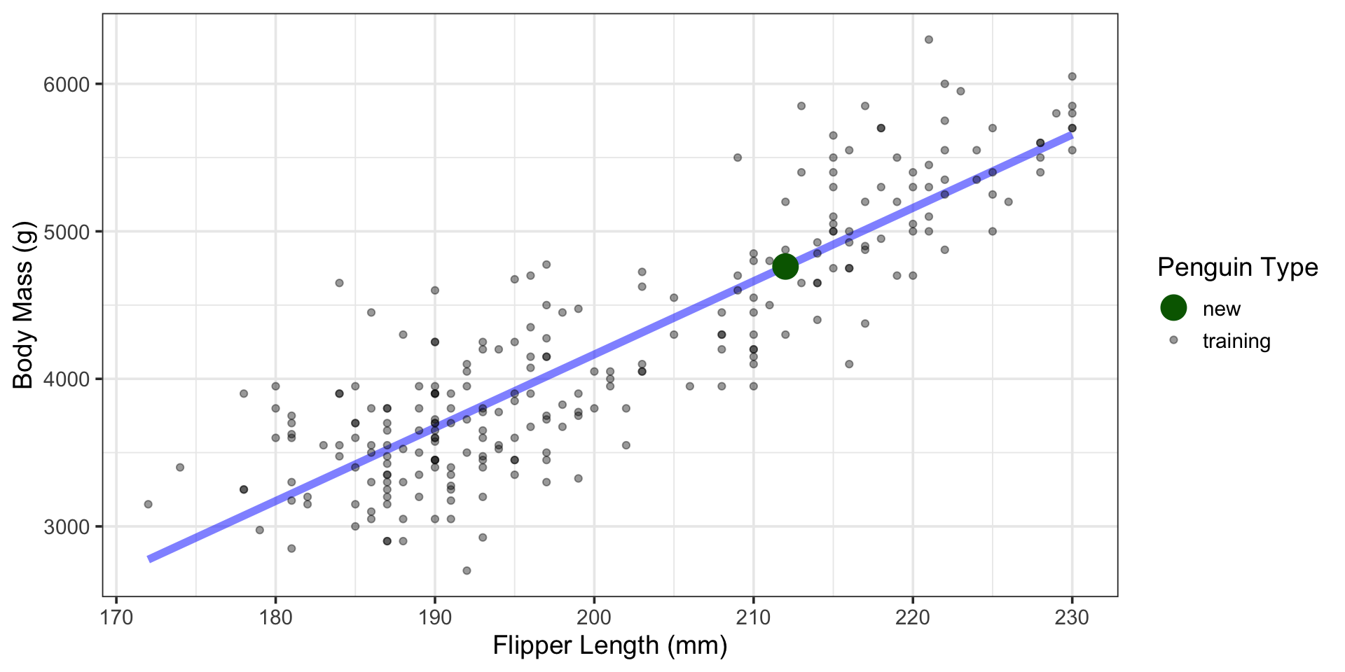
Using the Model to Make Predictions

new_penguin <- tibble(
  flipper_length_mm = 212
)

lin_reg_flip_fit %>%
  predict(new_penguin)

.pred
4761.638

Using the Model to Make Predictions

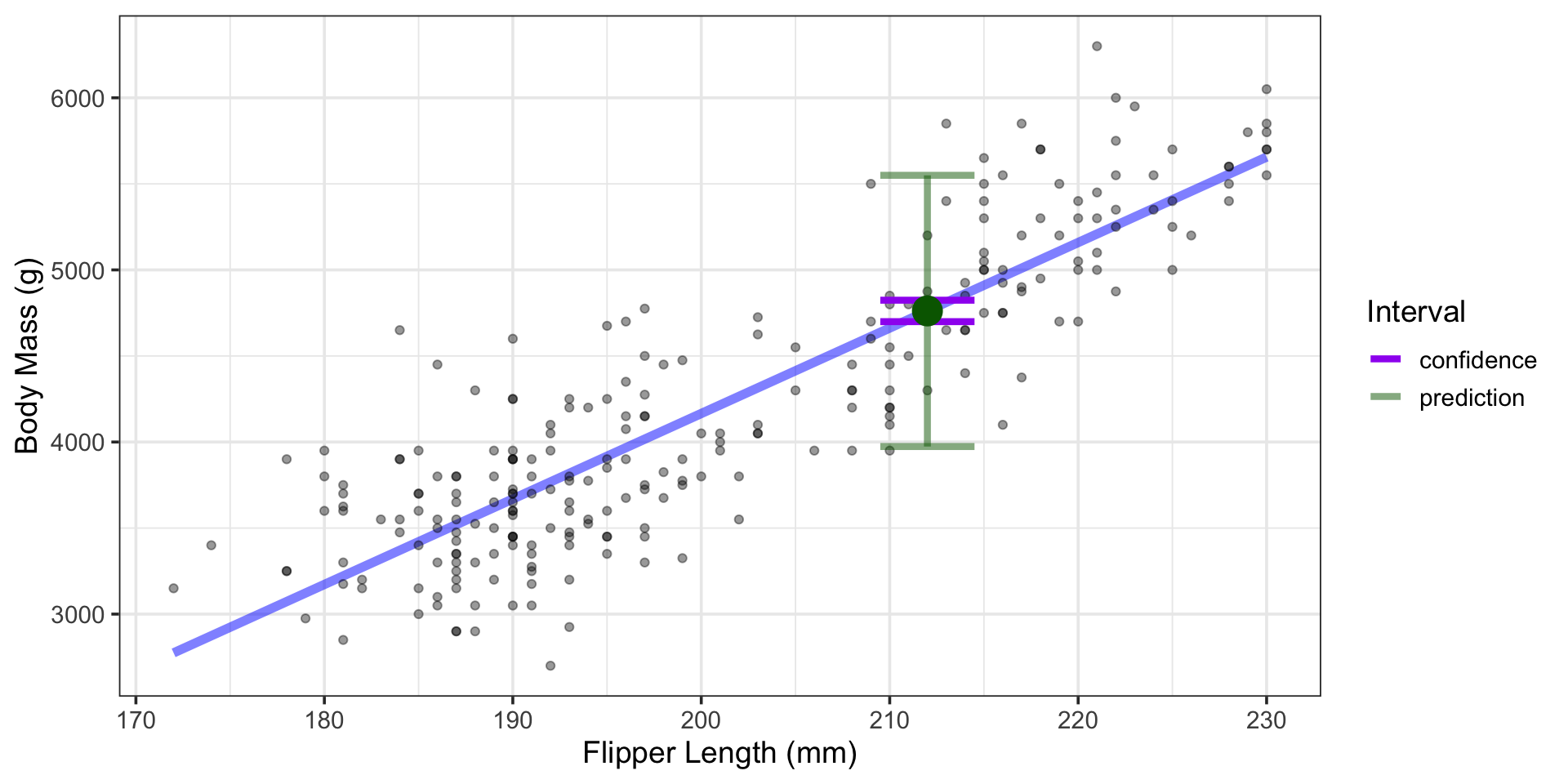
What is the body mass of a penguin whose flipper length is 212mm?

lin_reg_flip_fit %>%
  predict(new_penguin, 
          type = "pred_int", 
          level = 0.95)

.pred_lower	.pred_upper
3973.645	5549.631

Using the Model to Make Predictions

What is the average body mass of all penguins whose flipper length is 212mm?

lin_reg_flip_fit %>%
  predict(new_penguin, type = "conf_int", level = 0.95)

.pred_lower	.pred_upper
4699.363	4823.913

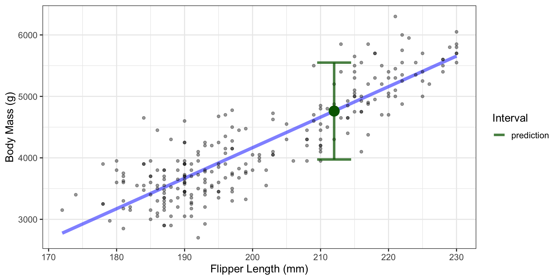
Using the Model to Make Predictions

What is the body mass of a penguin whose flipper length is 212mm?

• Somewhere between 3973.6g and 5549.6g, with 95% confidence.

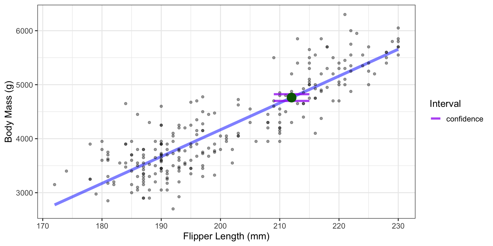
What is the average body mass of all penguins whose flipper length is 212mm?

• Somewhere between 4699.4g and 4823.9g, with 95% confidence.

Using the Model to Make Predictions

Let’s try this!

1. Write down two predictive questions associated with Air BnB rental prices that could be answered with your model

2. Can you differentiate versions of those questions that could be answered by confidence versus prediction intervals? What is the difference?

3. Compute your model’s prediction for a particular value of the predictor you chose

4. Similarly, compute the lower and upper bounds for bound confidence and prediction intervals for your chosen value

5. (Challenge) Can you plot the result?

6. Interpret your model’s predictions

   • Clearly differentiate the model prediction, versus the bounds for the confidence interval, versus the bounds for the prediction interval

Summary

• Simple linear regression models are models of the form \(\displaystyle{\mathbb{E}\left[y\right] = \beta_0 + \beta_1 x}\), with one predictor.
• We assume that the sole predictor is linearly associated with the response, independent of any other features.
• The global test for model utility and the test for significance of the predictor are identical in this case.
• We further assess simple linear regression models with summary metrics like \(R^2_{\text{adj}}\), RMSE (both training and testing), as well as residual plots.
• The intercept is the expected response when the predictor takes a value of 0, which may not be meaningful or supported.
• The coefficient on the predictor can be interpreted as a slope.
• We can predict responses for a single observation, or an average over all observations having the same value of the predictor.