As we discuss the different hypothesis test and interval analyses we’ll be encountering in the regression context, analyze the corresponding items for your models in that notebook
Does our model contain any useful information about predicting/explaining our response variable at all?
Hypotheses:
\[\begin{array}{lcl} H_0 & : & \beta_1 = \beta_2 = \cdots = \beta_k = 0\\
H_a & : & \text{At least one } \beta_i \text{ is non-zero}\end{array}\]
lin_reg_fit %>%glance()
r.squared
adj.r.squared
sigma
statistic
p.value
df
logLik
AIC
BIC
deviance
df.residual
nobs
0.7834185
0.7579384
6.253346
30.7462
2.3e-06
2
-63.41591
134.8318
138.8148
664.7737
17
20
Result: Since our \(p\) value is less than \(0.05\) (it’s about \(2.3 \times 10^{-6}\)), we reject the null hypothesis and accept that at least one of the terms in our model has a non-zero coefficient.
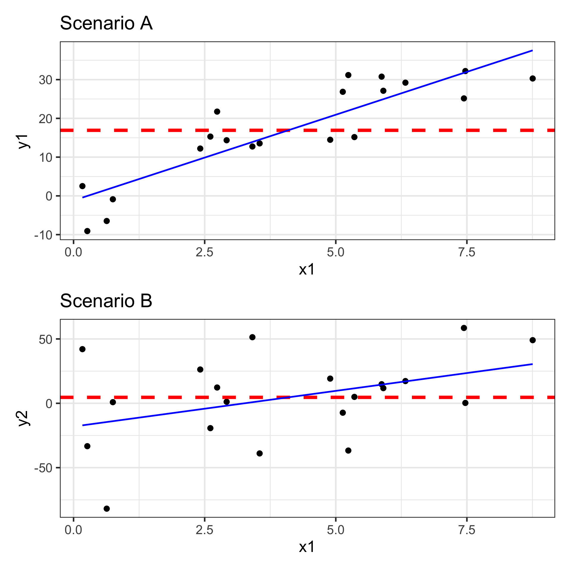
Global Test for Model Utility in Pictures
\[\begin{array}{lcl} H_0 & : & \beta_1 = \beta_2 = \cdots = \beta_k = 0\\
H_a & : & \text{At least one } \beta_i \text{ is non-zero}\end{array}\]
Are our sloped models better (more justifiable) models than the horizontal line?
Sloped models use predictor information
Horizontal models just predict average response, ignoring all observation-specific features
They assume that having information about features of an observation gives no advantage in predicting/explaining its response
Additional Global Metrics from glance()
lin_reg_fit %>%glance()
r.squared
adj.r.squared
sigma
statistic
p.value
df
logLik
AIC
BIC
deviance
df.residual
nobs
0.7834185
0.7579384
6.253346
30.7462
2.3e-06
2
-63.41591
134.8318
138.8148
664.7737
17
20
The output from glance()ing at our fitted model object gives lots of additional information about overall model fit and quality.
The adjusted R-squared value (adj.r.squared) measures the proportion of variation in the response variable which is explained by the terms in our fitted model.
The adjusted R-squared value is a better measure than R-squared because adjusted R-squared penalizes the inclusion of additional model terms.
The sigma value is our residual standard error, which we’ll often call our “training error”. It is a measure of how far off we should expect our predictions to be, on average (but it is a biased measure).
We won’t generally consider the additional items in our course.
Result: The x1 predictor is statistically significant but the x2 predictor is not. We should drop the x2 predictor from the model and re-fit it. (\(\bigstar\) We’ll only ever drop one predictor / model term at a time, using the highest p-value to indicate which.)
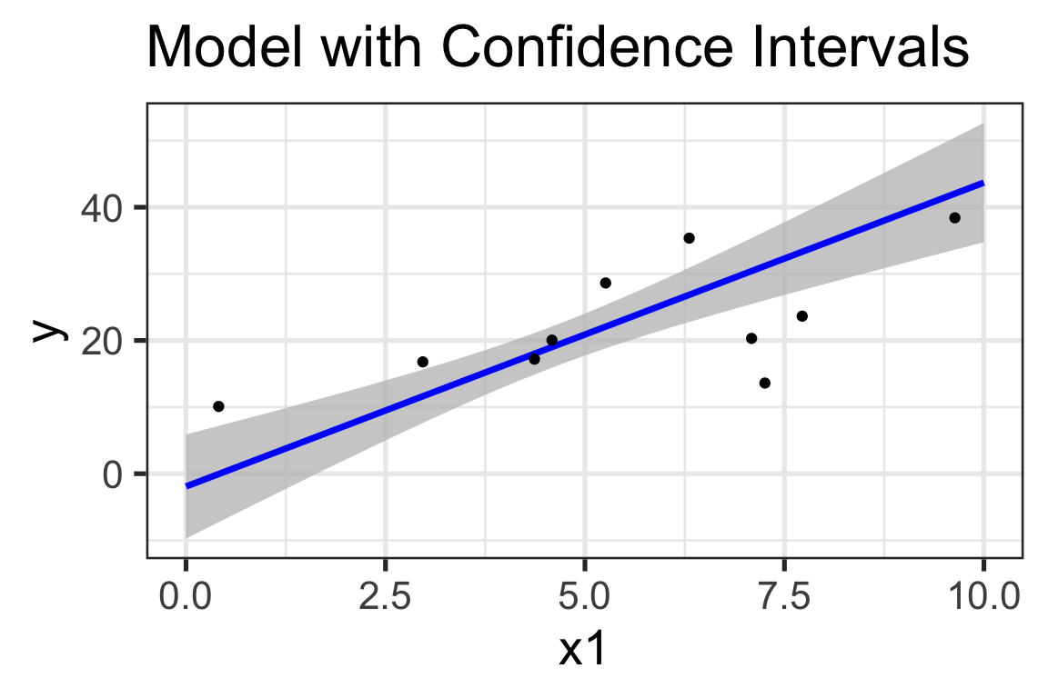
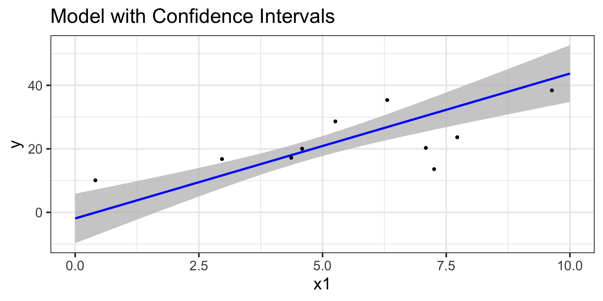
Confidence Intervals (Model Coefficients)
Reminder: An approximate 95% confidence interval is between two standard errors below and above our point estimate.
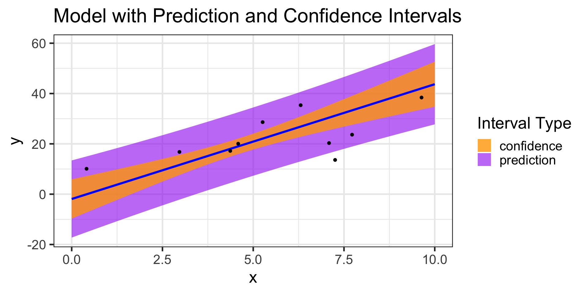
Are these wrong too? No – confidence intervals bound the average response over all observations having given input features.
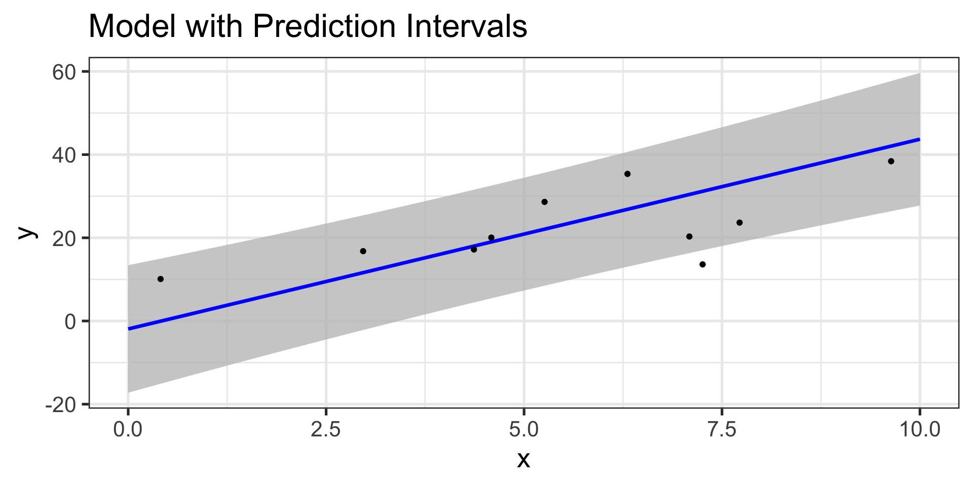
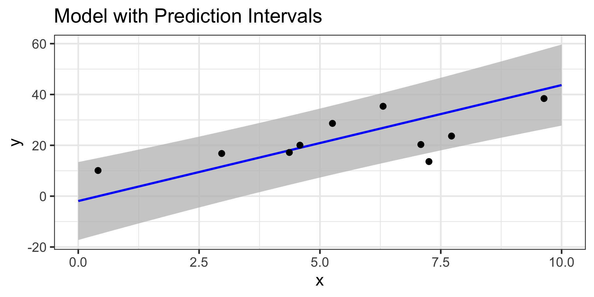
Prediction Intervals
So, can we build intervals which contain predictions on the level of an individual observation?
Sure – but there’s added uncertainty in making those types of predictions
Confidence and Prediction Intervals for Model Predictions
Summary
Below are the most common applications of statistical inference in regression modeling.
Hypothesis Tests
Does our model have any utility at all?
Are all of the included predictor terms useful?
Confidence Intervals
What is the plausible range for each parameter/coefficient?
How do we interpret those ranges?
Can we make reliable predictions?
Confidence Intervals for average response
Prediction Intervals for individual response
We’ll be utilizing all of these ideas throughout our course.
We’ll leverage R functionality to obtain intervals or to calculate test statistics and \(p\)-values though, since it is much faster than doing any of this by hand.
Next Time…
Hypothesizing, Constructing, Assessing, and Interpreting Simple Linear Regression Models