{tidymodels} Overview
September 24, 2024
A Reminder About Our Goals
So…how do we do it?
The Highlights
Obtain training and validation data
Build a model using the
{tidymodels}framework- Model specification (declaring the type of model)
- Recipe (defining the response, features, and transformations)
- Workflow (encapsulate the specification and recipe together)
- Fit the workflow to training data
Assess model performance
- Global performance metrics (training data)
- Individual term-based assessments (training data)
- We’ll add more assessment techniques later
Making predictions
Splitting Training and Test Data
set.seed(080724) #set seed for reproducibility

data_splits <- my_data %>% #begin with `my_data` data frame
  initial_split(prop = 0.75) #split into 75% train / 25% test

train <- training(data_splits) #collect training rows into data frame
test <- testing(data_splits) #collect validation rows into data frame
Make sure to always set a seed. It ensures that you obtain the same training and testing data each time you run your notebook/model.
\(\bigstar\) Let’s try it! \(\bigstar\)
- Open RStudio and your MAT300 project
- Open the Notebook you had been using to explore our AirBnB Europe data from two weeks ago.
- Save a new copy of it, perhaps named
MyModelingNotebook.qmd. - Keep the YAML Header (but update the title) and keep the first code chunk – the one that (i) loads your packages, (ii) reads in the AirBnB data, and (iii) cleans up the column names, but delete everything below it.
- Add code to load the
{tidymodels}package into your notebook, if it is not already loaded. - Adapt the code on this slide to split your
airbnbdata intotraining andtestsets.
Build and Fit a Model
lin_reg_spec <- linear_reg() %>% #define model class
  set_engine("lm") #set fitting engine

#Set recipe, including response and predictors
#Predictors are separate by "+" signs
lin_reg_rec <- recipe(response ~ pred_1 + pred_2 + ... + pred_k,
                      data = train)

lin_reg_wf <- workflow() %>% #create workflow
  add_model(lin_reg_spec) %>% #add the model specification
  add_recipe(lin_reg_rec) #add the recipe

#Fit the workflow to the training data
lin_reg_fit <- lin_reg_wf %>%
  fit(train)
\(\bigstar\) Let’s try it! \(\bigstar\)
- Construct a linear regression model specification
- Choose a few of the available (numeric) predictors of listing price for the
airbnbrentals in your data set and construct a recipe to predict price using those predictors - Package your model and recipe together into a workflow
- Fit the workflow to your training data
Global Model Assessment on Training Data
| metric | values |
|---|---|
| r.squared | 0.7595231 |
| adj.r.squared | 0.7538648 |
| sigma | 3.1320329 |
| statistic | 134.2321602 |
| p.value | 0.0000000 |
| df | 4.0000000 |
| logLik | -445.5722346 |
| AIC | 903.1444693 |
| BIC | 922.1331851 |
| deviance | 1667.6371409 |
| df.residual | 170.0000000 |
| nobs | 175.0000000 |
Term-Based Assessments
| term | estimate | std.error | statistic | p.value |
|---|---|---|---|---|
| (Intercept) | 33.884098 | 1.3207624 | 25.654954 | 0.0000000 |
| displ | -1.259214 | 0.5772141 | -2.181536 | 0.0305166 |
| cyl | -1.516722 | 0.4182149 | -3.626658 | 0.0003793 |
| drv_f | 5.089640 | 0.6514639 | 7.812621 | 0.0000000 |
| drv_r | 5.046396 | 0.8205130 | 6.150294 | 0.0000000 |
You can conduct inference and interpret model coefficients from here as well!
\(\bigstar\) Let’s try it! \(\bigstar\)
- Extract the term-based model assessment metrics from your fitted model object
- Pay special attention to the
estimate,std.error, andp.valuecolumns of the output – what can you use these for?
Making Predictions
We can obtain predictions using two methods, as long as the new_data you are predicting on includes all of the features from your recipe().
To create a single column (.pred) data frame of predictions or columns of lower and upper interval bounds.
Note: Your “new data” could be your training data, your testing data, some new real observations that you want to make predictions for, or even some counterfactual (hypothetical) data
Making Predictions
\(\bigstar\) Let’s try this! \(\bigstar\)
- Use
predict()to make predictions for the rental prices of your training observations, then useaugment()to do the same – what is the difference? - Plot your model’s predictions with respect to one of your predictor variables.
If you are successful doing the above…
- Find the minimum (
MIN_VAL) and maximum (MAX_VAL) observed training values for one of your numeric predictors - Create a
new_datadata frame usingtibble()andseq().- Include a column for each of the predictors your model uses – be sure to use the exact same names as in your
training set - Choose a fixed value for all but your selected numerical variable (they could be different from one another)
- For your chosen variable, use
seq(MIN_VAL, MAX_VAL, length.out = 250)
- Include a column for each of the predictors your model uses – be sure to use the exact same names as in your
- Use
predict()andaugment()to make price predictions for these fictitious (counterfactual) rentals- Can you get interval bounds rather than predictions using
predict()?
- Can you get interval bounds rather than predictions using
Additional Tasks
Build a simpler model, one using just a single numerical predictor. Then, for this model, try each of the following…
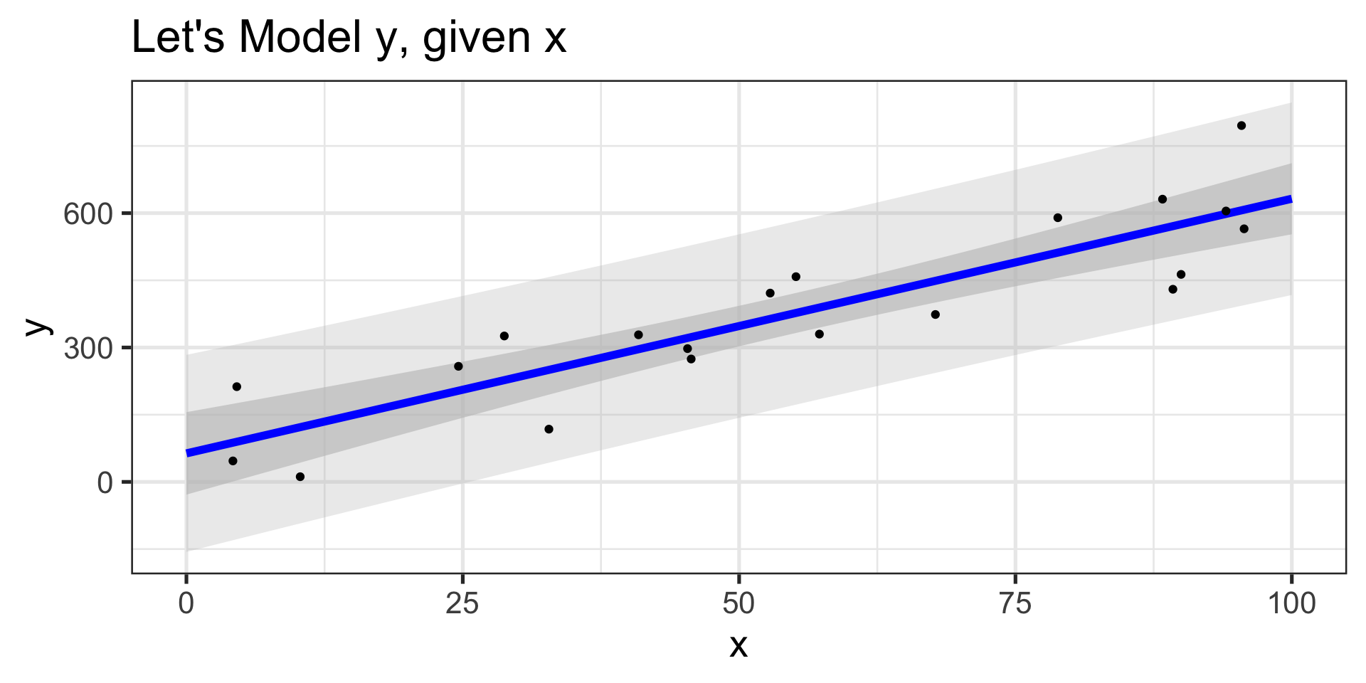
Plotting and interpreting model predictions
- A scatterplot of the original training data
- A lineplot showing the model’s predictions
- An interval band showing the confidence intervals for predictions (hint. use
geom_ribbon()) - An interval band showng the prediction intervals for predictions
- Meaningful plot labels
- Interpret the resulting plot
Do you have a preference for the order in which you include the geometry layers?
Calculating and analysing training residuals
- Can you add a column of predictions to your training data set?
- Can you mutate a new column of prediction errors (residuals) onto your training data set?
- Can you plot a histogram and/or density plot of the residuals?
- Analyse the plot you just created – what do you notice? Is this what you expected?
Next Time…
A review of hypothesis testing and confidence intervals