Overview of Statistical Learning (and Competition Overview)

Dr. Gilbert

September 6, 2024

Statistical Learning in Pictures

Statistical Learning in Pictures

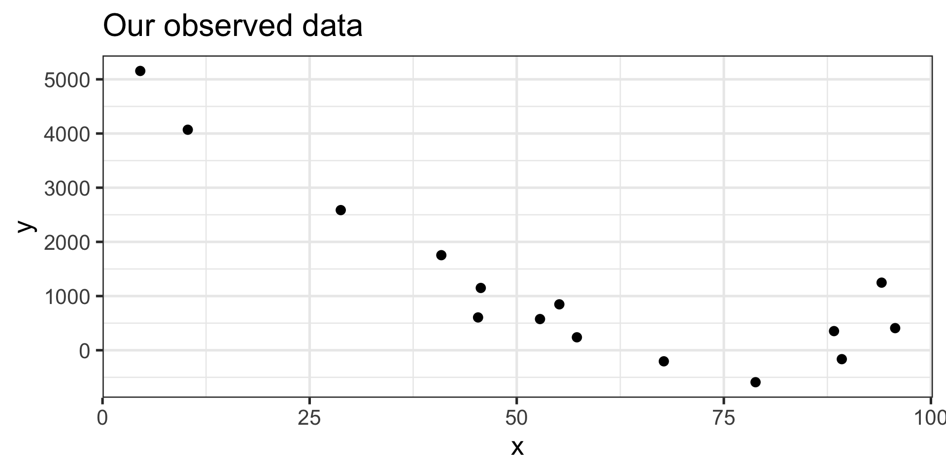
Goal: Build a model \(\displaystyle{\mathbb{E}\left[y\right] = \beta_0 + \beta_1 x}\) to predict \(y\), given \(x\).
Generalized Goal: Build a model \(\displaystyle{\mathbb{E}\left[y\right] = \beta_0 + \beta_1 x_1 + \beta_2 x_2 + \cdots + \beta_k x_k}\) to predict \(y\) given features \(x_1, \cdots, x_k\).
- \(\beta_i\)’s are parameters, learned from training data.

Statistical Learning in Pictures

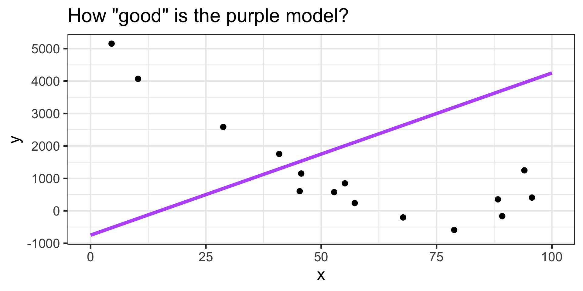
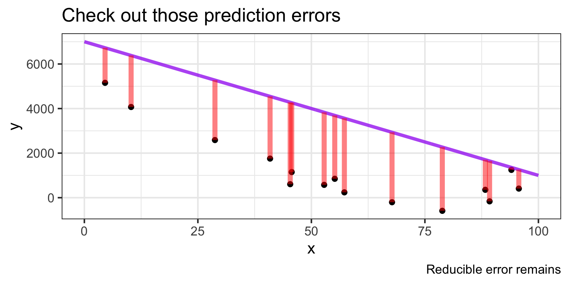
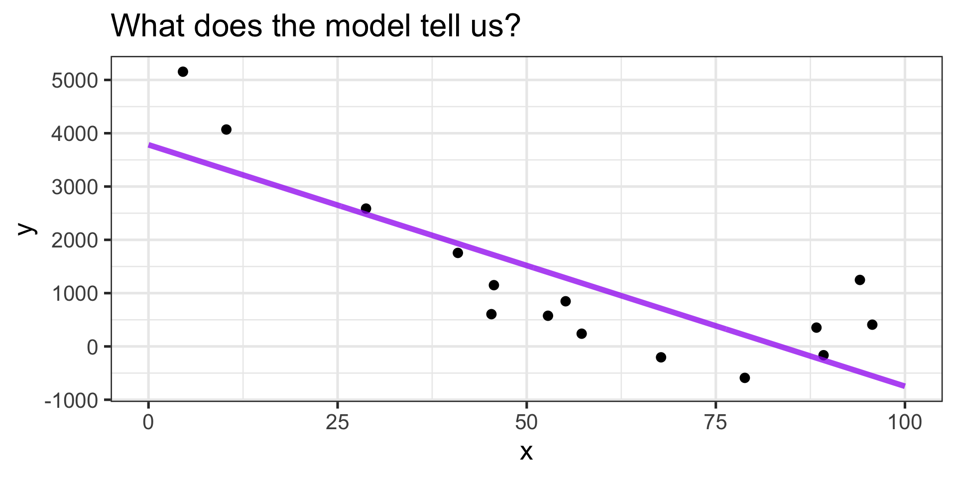
This model doesn’t capture the general trend between our observed \(x\) and \(y\) pairs.

Statistical Learning in Pictures

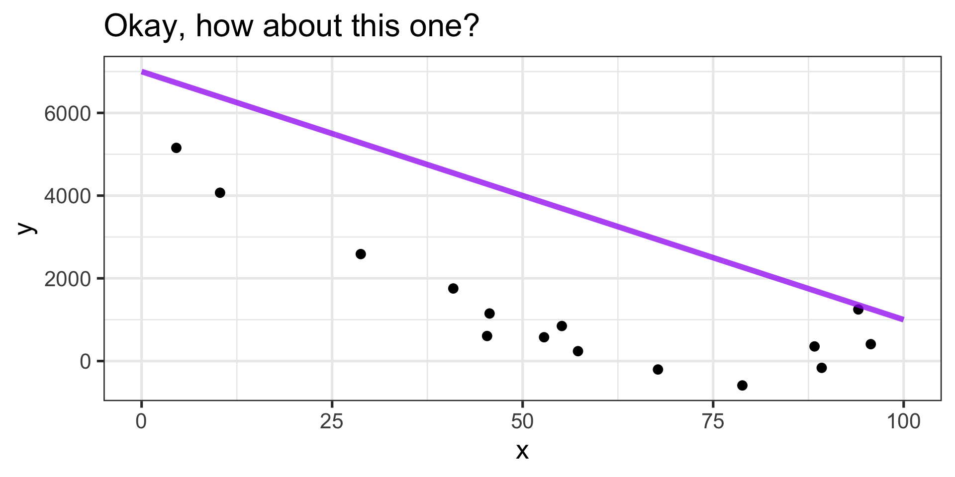
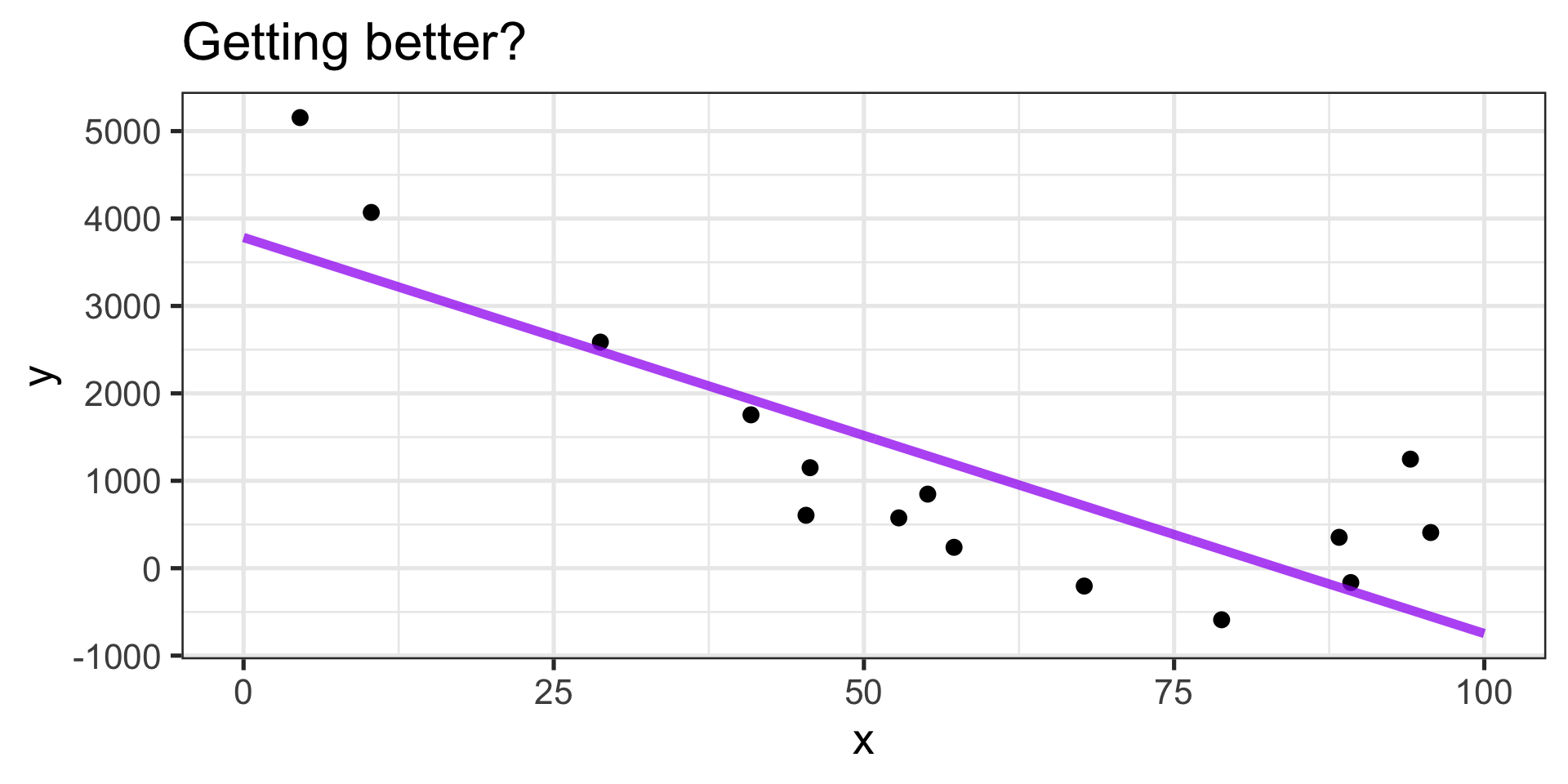
Better job capturing the general trend (sort of).
Larger \(x\) values are associated with smaller \(y\) values.

Statistical Learning in Pictures

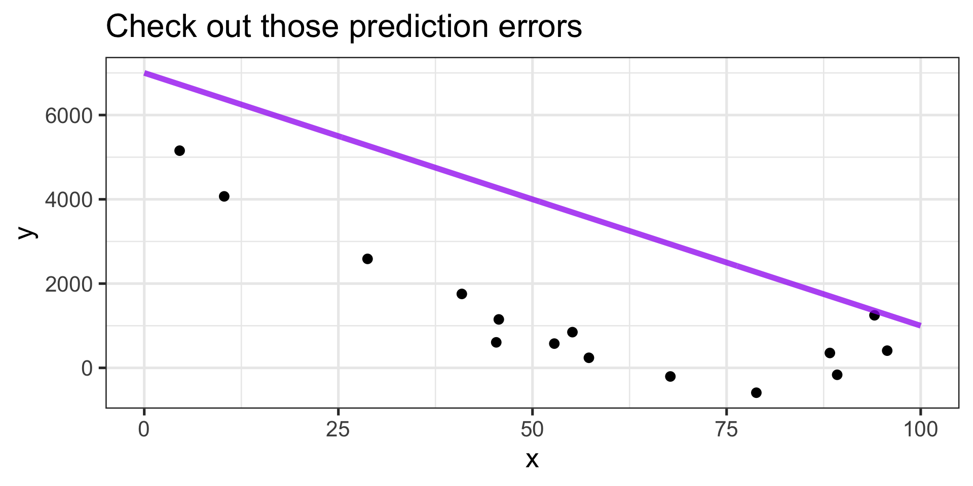
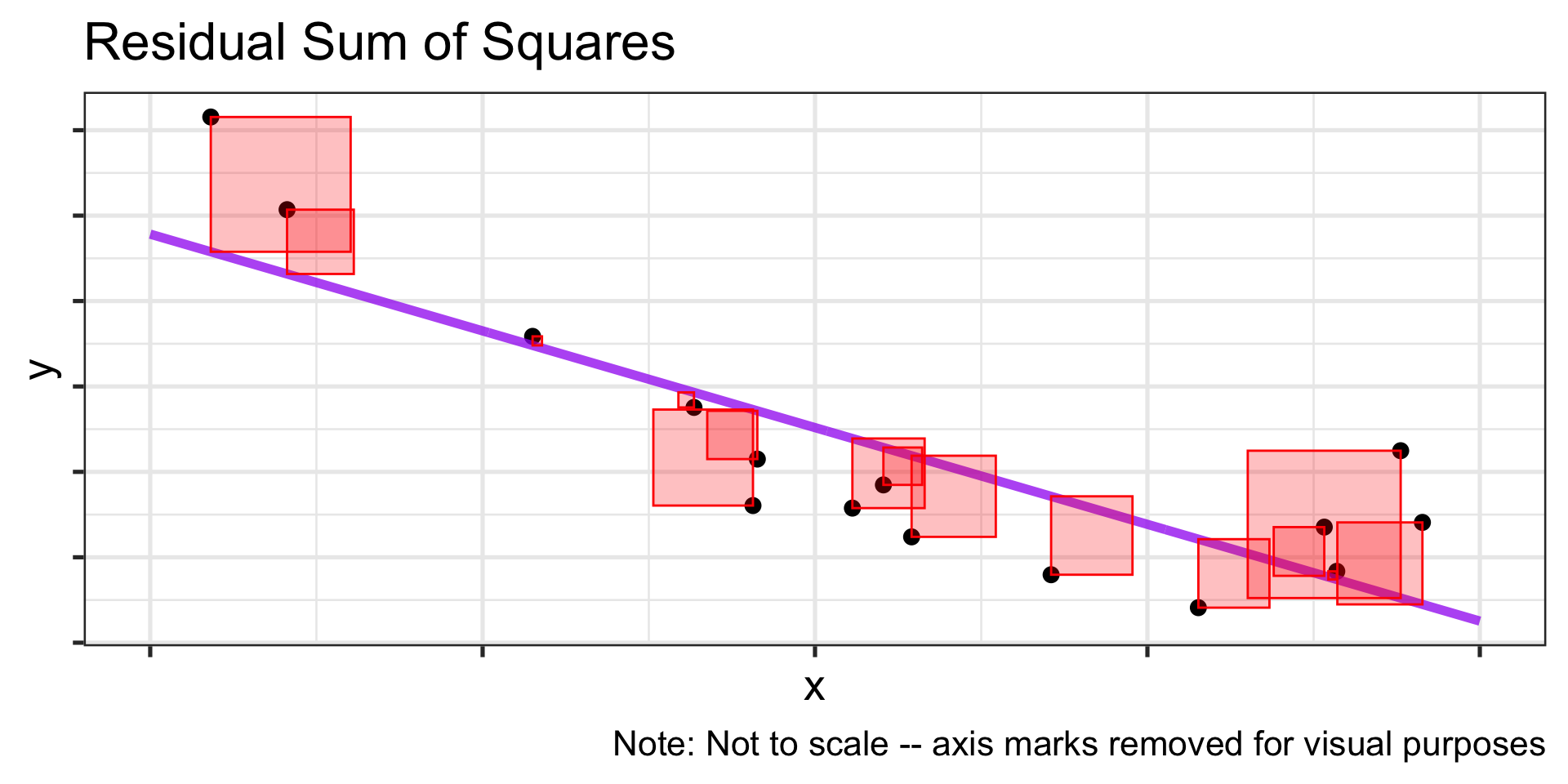
Always predicting too high!
- We should overpredict sometimes and underpredict others. The average error should be \(0\).

Statistical Learning in Pictures

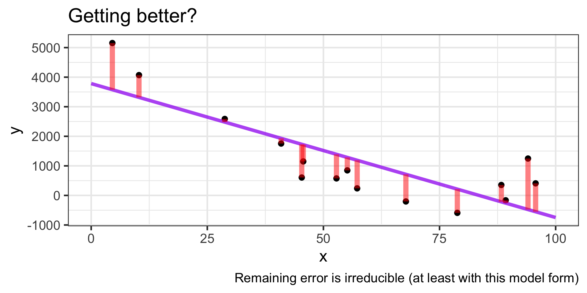
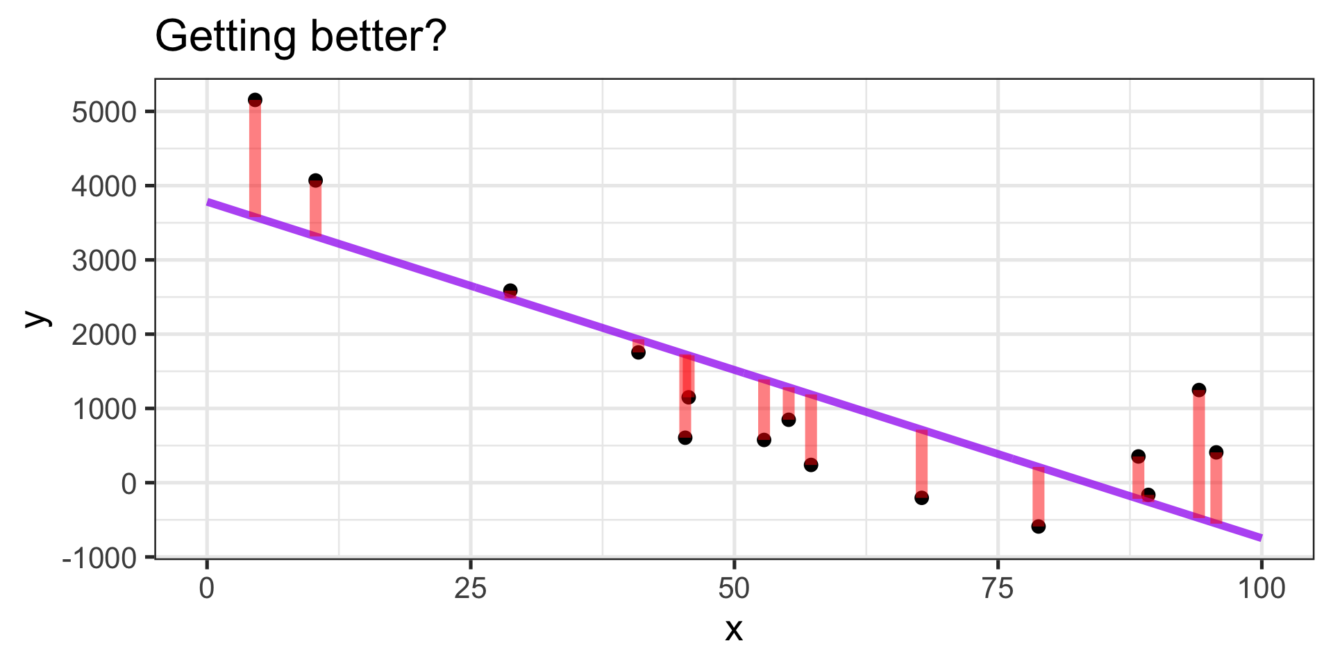
Capturing the general trend?
- …mostly
Balanced errors?
- ✓

How it works

In this case, we have \(\mathbb{E}\left[y\right] = \beta_0 + \beta_1\cdot x\) and we find \(\beta_0\) (intercept) and \(\beta_1\) (slope) to minimize the quantity

\[\sum_{i = 1}^{n}{\left(y_{\text{obs}_i} - y_{\text{pred}_i}\right)^2}\]

How it works

In this case, we have \(\mathbb{E}\left[y\right] = \beta_0 + \beta_1\cdot x\) and we find \(\beta_0\) (intercept) and \(\beta_1\) (slope) to minimize the quantity

\[\sum_{i = 1}^{n}{\left(y_{\text{obs}_i} - \left(\beta_0 + \beta_1\cdot x_{\text{obs}_i}\right)\right)^2}\]

Changing \(\beta_0\) and/or \(\beta_1\) will change this sum.

How it works

Interpreting the Model

\(\displaystyle{\mathbb{E}\left[y\right] = 3783.21 - 45.3\cdot x}\)

The expected value of \(y\) when \(x = 0\) is \(3783.21\).
As \(x\) increases, we expect \(y\) to decrease (on average).
Given a unit increase in \(x\), we expect \(y\) to decrease by about \(45.3\) units.

Interpreting the Model

\(\displaystyle{\mathbb{E}\left[y\right] = 3783.21 - 45.3\cdot x}\)

The expected value of \(y\) when \(x = 0\) is \(3783.21\).
As \(x\) increases, we expect \(y\) to decrease (on average).
Given a unit increase in \(x\), we expect \(y\) to decrease by about \(45.3\) units.

Approach to Model Interpretation: In general, we’ll interpret the intercept (when appropriate) and the expected effect of a unit change in each predictor on the response

Can we find a better model?

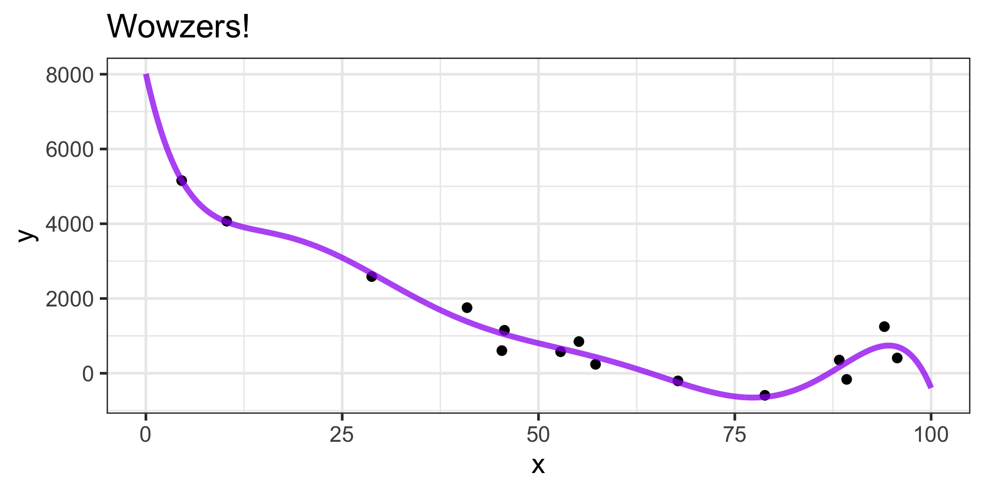
Can we interpret this model?

The equation is \(\mathbb{E}\left[y\right] \approx 1202 - 4911x +3156x^2 + 784x^3 +\\ 409x^4 -215x^5 -7x^6 -516x^7\)
No thanks…

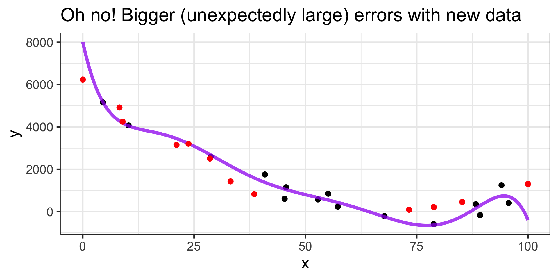
Do we expect this model to generalize well?

Especially near \(x = 0\) and \(x = 100\)

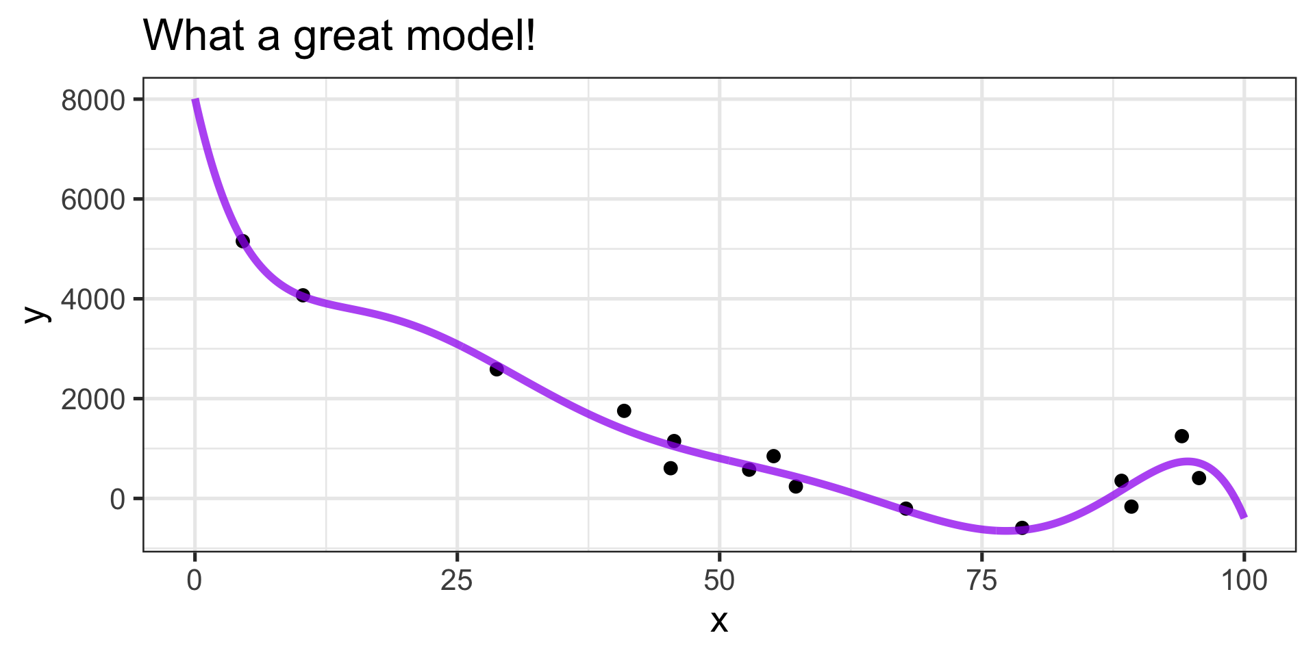
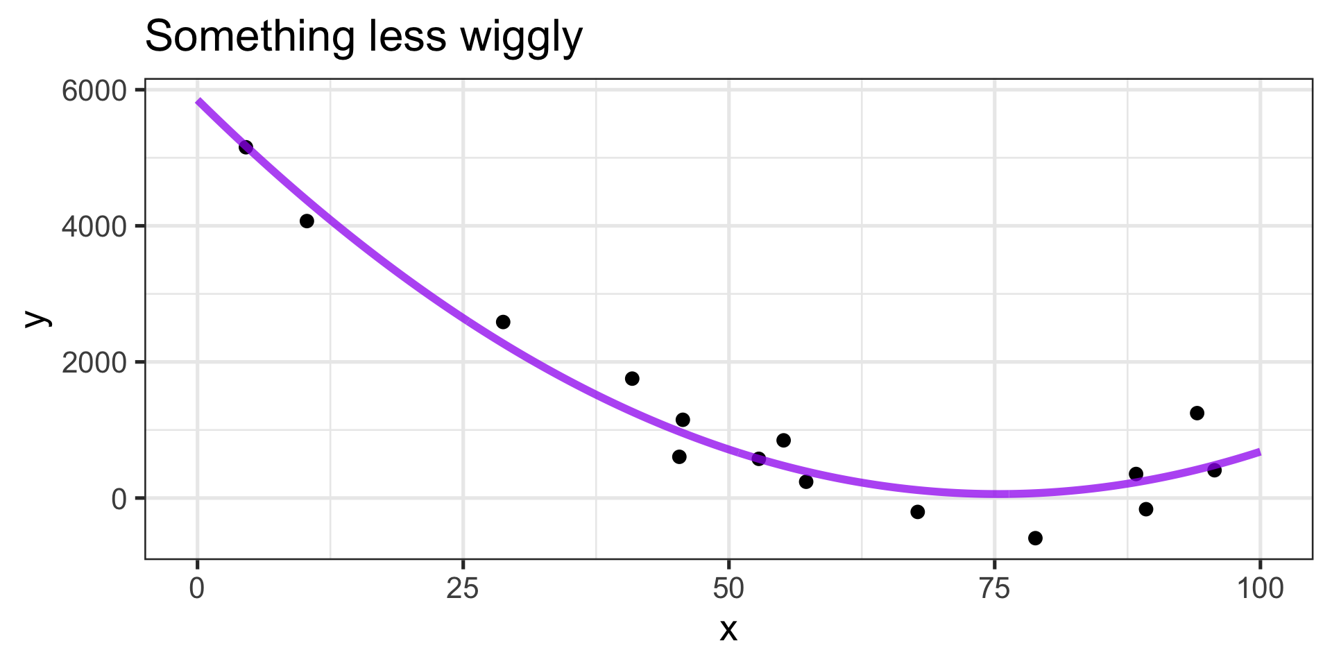
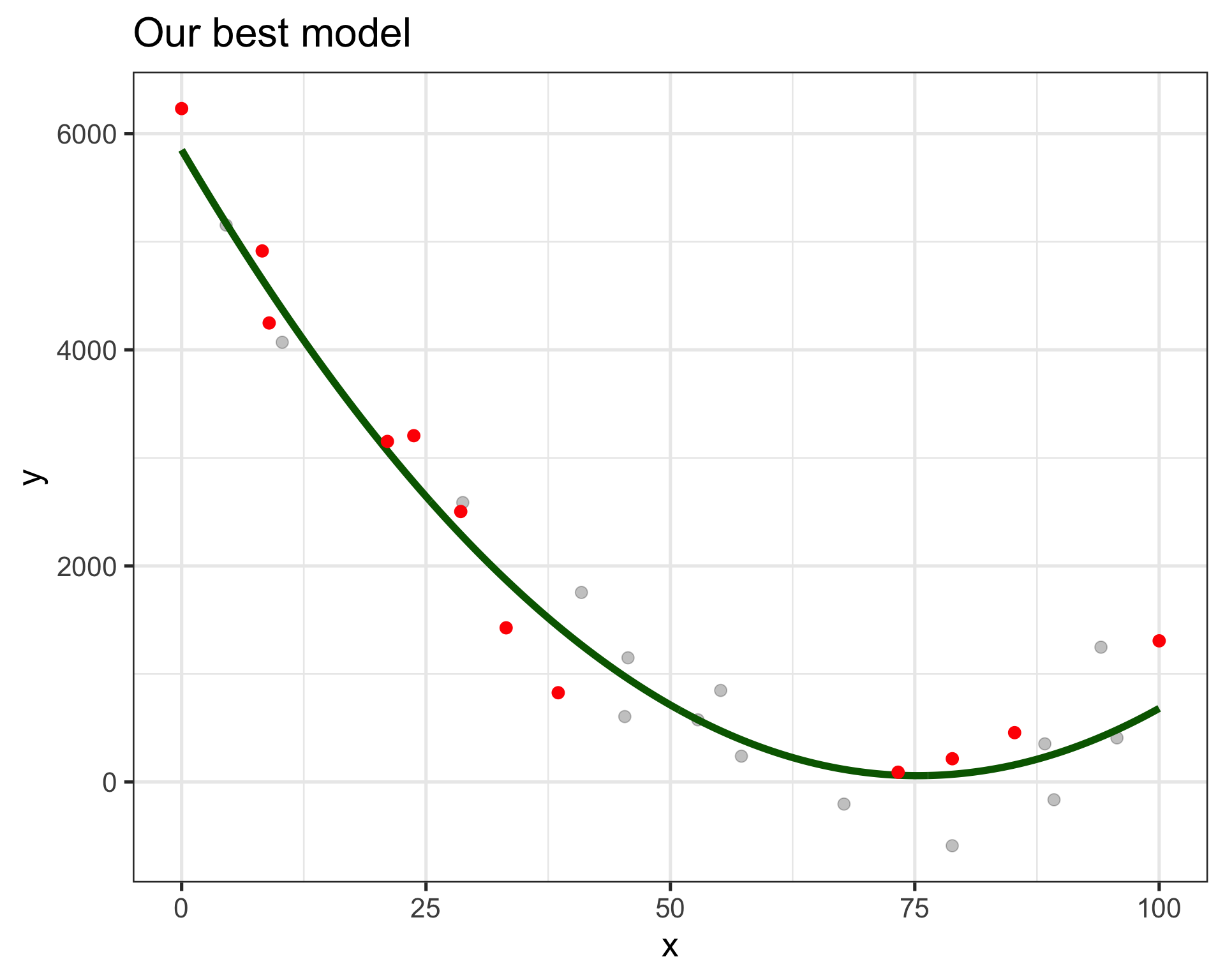
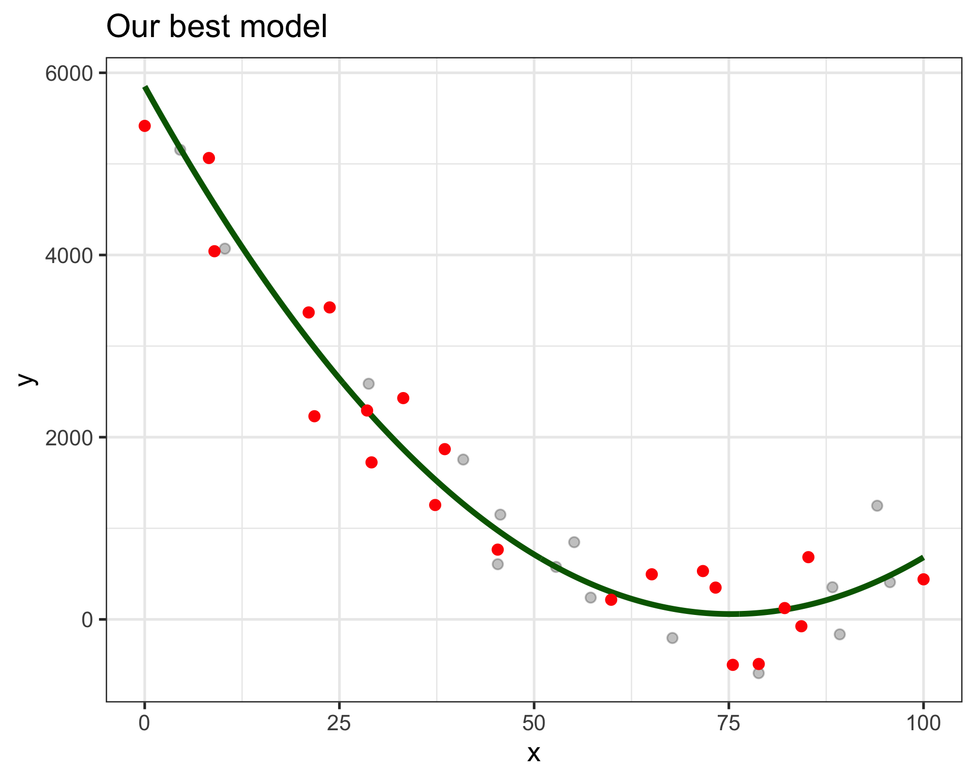
Is there a happy medium?

Is there a happy medium?

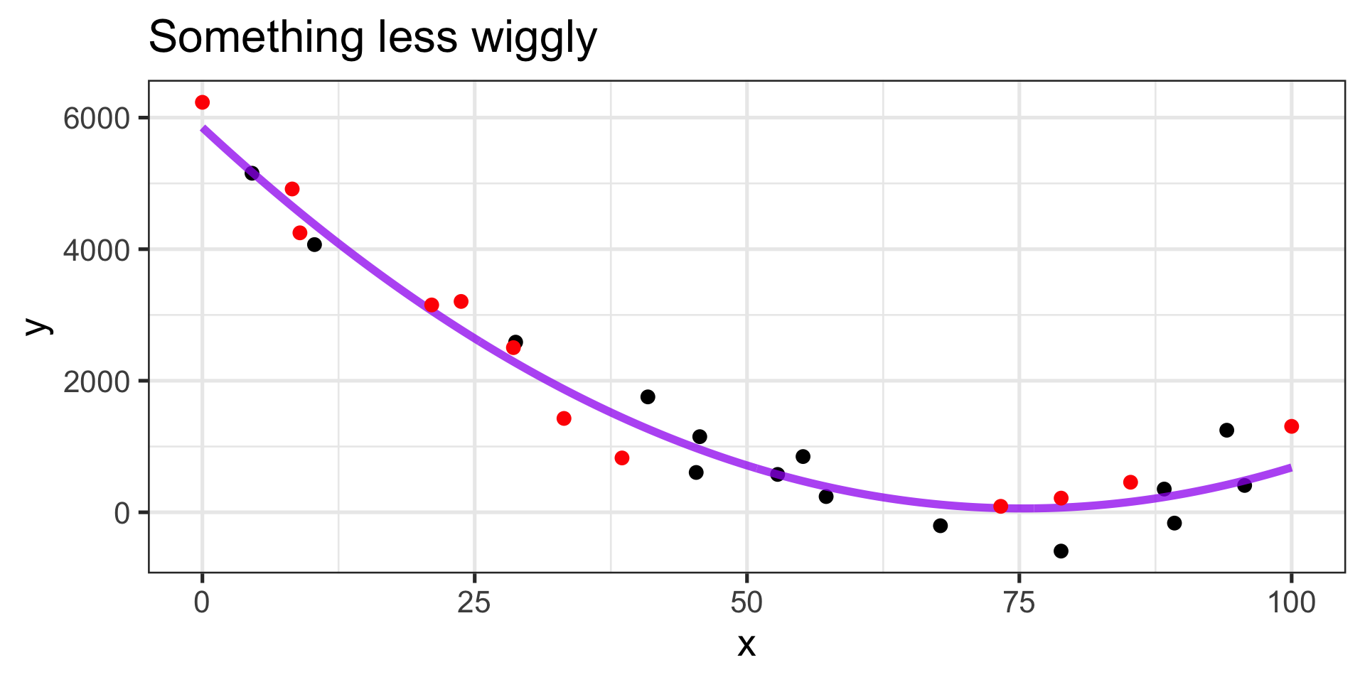
Fits old and new observations similarly well
Equation \(\displaystyle{\mathbb{E}\left[y\right] \approx 1202 -4912x + 3156x^2}\)
- We’ll be able to interpret this

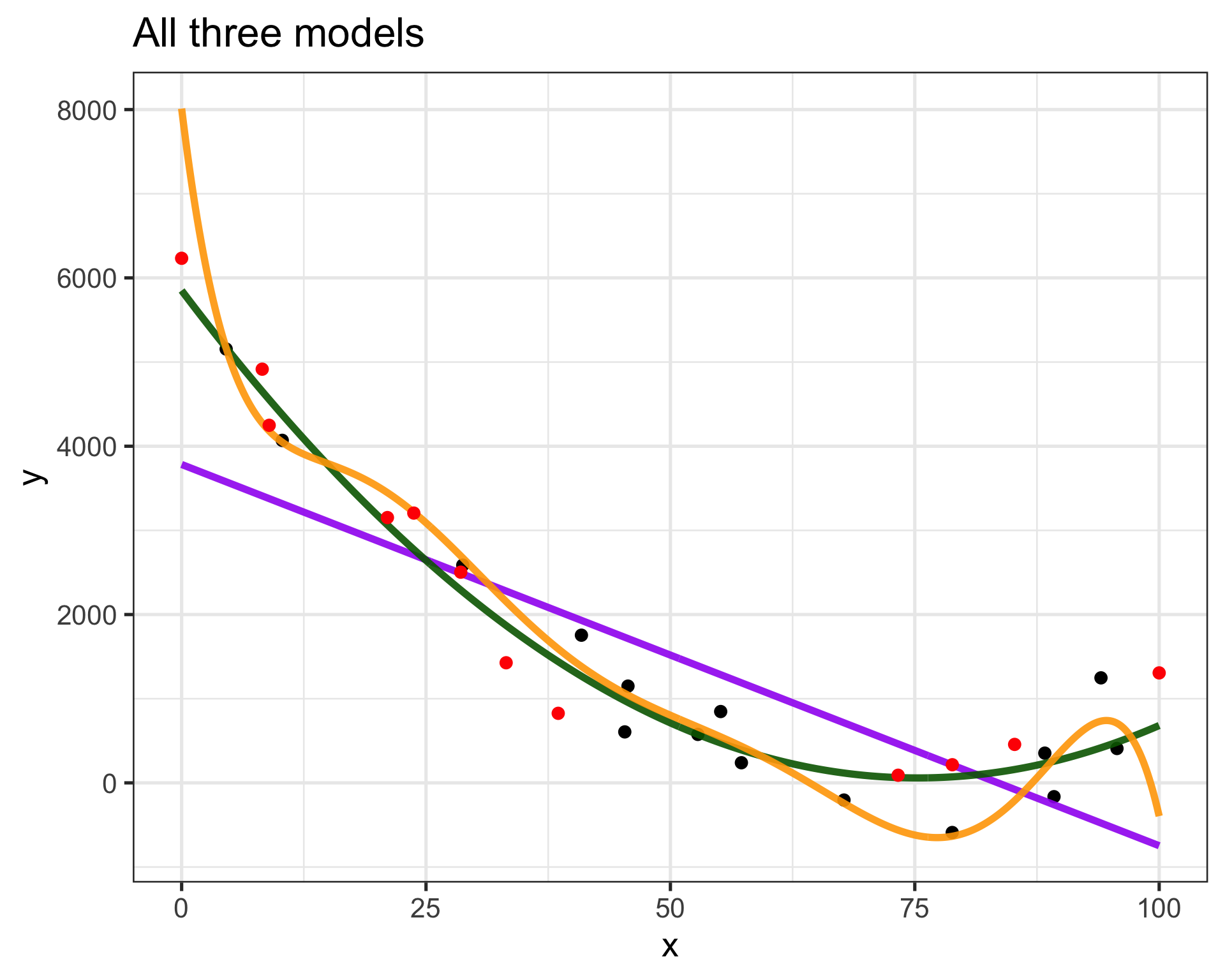
How do we know what model is right?

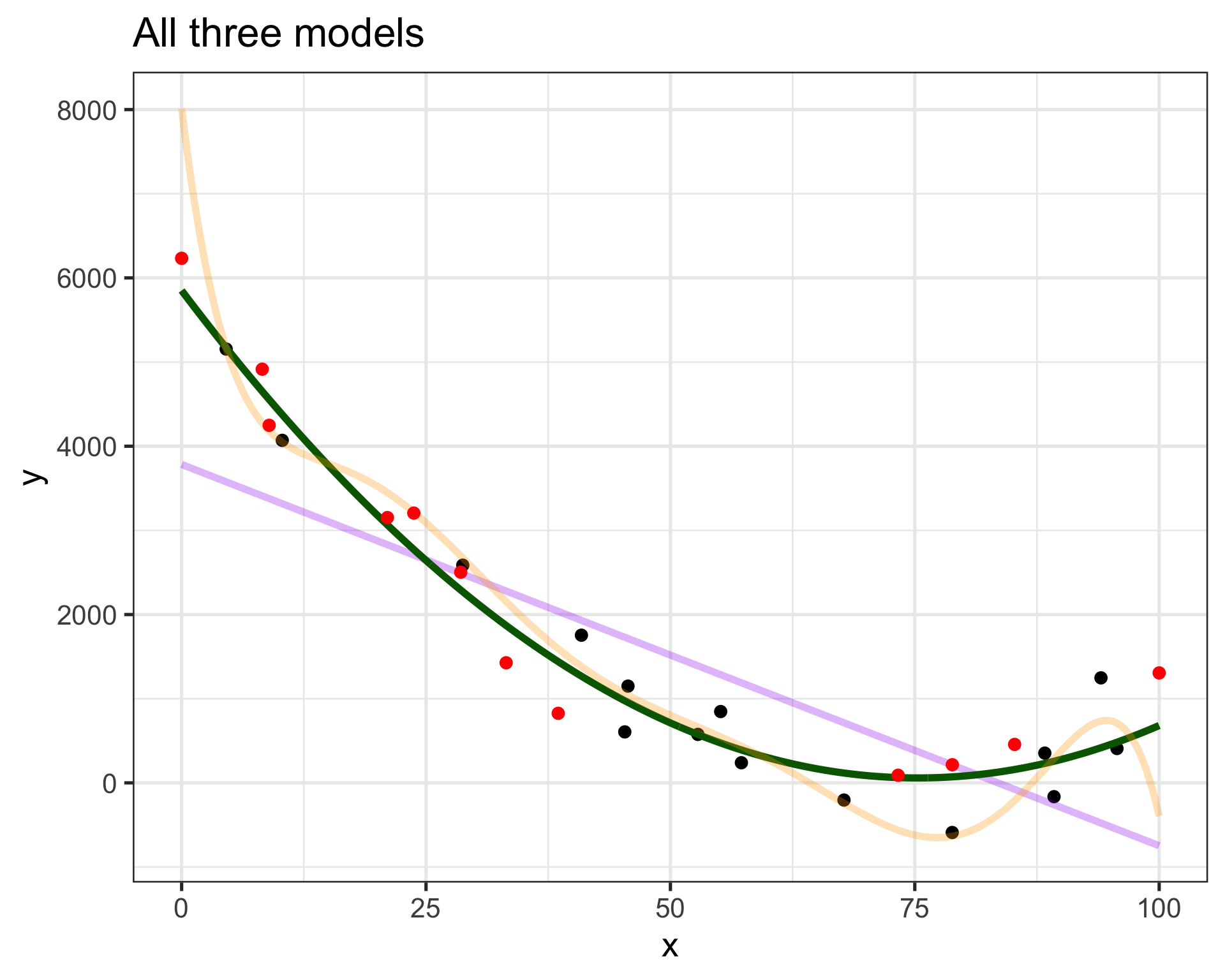
The purple model is too straight
The orange model is too wiggly
The green model is just right

How do we know what model is right?

We don’t want to wait for new data to know we are wrong.
- Use some of our available data for training
- And the rest for validation

Okay, but our predictions are all wrong…literally!

All models are wrong, but some are useful, George Box (1976)
Predictions will be wrong but, with some assumptions, they have value

Necessary Assumptions

For model and predictions

Training data are random and representative of population.
- Otherwise, we should not be modeling this way.
Residuals (prediction errors) are normally distributed with mean \(\mu = 0\) and constant standard deviation \(\sigma\).
- Allows construction of confidence intervals around predictions (making our models right).

Necessary Assumptions

For interpretations of coefficients (statistical learning / inference)

No multicollinearity (predictors aren’t correlated with one another)

Summary

Building models \(\mathbb{E}\left[y\right] = \beta_0 + \beta_1 x_1 + \beta_2 x_2 + \cdots + \beta_k x_k\)
Predicting a numerical response (\(y\)) given features (\(x_i\))
Need data to build the models – some for training, some for validation
- The \(\beta_i\)’s are parameters whose values are learned/estimated from training data
Model predictions will be wrong
As long as standard deviation of residuals (prediction errors) is constant, we can build meaningful confidence intervals for predictions
Can interpret models to gain insight into relationships between predictor(s) and response

Competition Information

Predict Door Dash delivery times
- Time from placing order to delivery
Response: delivery time
Predictors: market_id, order_time, delivery_time, store_id, cuisine_type, order_protocol, items_in_order, subtotal_cost, distinct_items_in_order, min_item_price, max_item_price, dashers_working, busy_dashers, outstanding_orders, model_1_estimate, model_2_estimate

How this works

Six assignments to guide you.
You’ll take data provided by Door Dash and build models.
Kaggle will assess the predictions from everyone’s models.
Live leaderboard, using only part of the competition data so you know approximately where you stand.
You’ll talk with eachother about why/how you have different scores.
People might share their strategies, or they might not – this is a competition after all.

Why?

Interest in homework assignments generally ends after they’re turned in and graded.
Competition assignments and environment ask you to iterate on previous work.
You’ll almost surely be interested in what other people have done, especially if their models have performed better than yours.
You’ll talk with eachother about strategies and modeling choices.
You’ll be motivated to improve your model even between assignments.

What past students say

The competition is fun
It is motivating
I learned more because I wanted to place better in the competition
Talking with others about their models made me more confident in my understanding of course material

What you are building

An analytics report
You’ll be building models and (more importantly) writing about your modeling choices and the performance of your models
Six assignments – each focusing on part(s) of the modeling process and analytics report
Prepares you for the final project, where you’ll do all this over again on a data set you identified and care about

Next Time…

Way fewer slides! 🤕
An introduction to R
Getting our hands dirty!

Homework: Start Competition Assignment 1 – join the competition, read the details, download the data, and start writing a Statement of Purpose