Hyperparameters and Tuning

Dr. Gilbert

September 1, 2024

Motivation

We’ve discussed several new model classes recently

With each class, we’ve been required to set model parameters manually, prior to the model seeing any data

Ridge Regression and LASSO:

  • mixture
  • penalty

Nearest Neighbor Regressors:

  • neighbors

Tree-Based Models:

  • max_depth

Ensembles (Random Forest, Boosted Trees):

  • mtry
  • trees
  • learn_rate
  • etc.

Every modeling choice we make should be justified…

How can we make justifiable choices for these parameters?

Model Hyperparameters

A hyperparameter is a model parameter (setting) that must be chosen prior to the model being fit to training data

That is, hyperparameters are set outside of the model fitting process

If these parameters need to be determined prior to seeing data, how can we optimize (or even justify) our choices?

Keep Calm, and …

Keep Calm, and Cross-Validate

I told you that cross-validation was useful for more than just estimating more stable performance estimates

With cross-validation, we can try multiple combinations of hyperparameter settings

The cross-validation procedure results in performance estimates (and standard error estimates) for each model and hyperparameter combination

From here, we can identify not only the best model, but also the best hyperparameter choices

We’ll call this process tuning

Playing Along

Again, we’ll continue with the ames data

  1. Open your notebook from our last two meetings
  2. Run all of the existing code
  3. Add a new section to your notebook on hyperparameters and model tuning

Tuning a Decision Tree Regressor

Decision tree regressors are a great first model class to tune because optimizing the max_depth parameter is intuitive

The deeper a decision tree, the more flexible it is, and the more likely it is to overfit

If a tree is too shallow though, it will be underfit

Let’s tune a tree to identify the optimal depth for predicting selling prices of homes in the Ames, Iowa data

Defining a Model with Tuning Parameters

Most of model tuning is done exactly as we approached assessing models robustly with cross-validation

The only difference is that we’ll indicate parameters to be tuned by setting them to tune()

dt_spec <- decision_tree(tree_depth = tune()) %>%
  set_engine("rpart") %>%
  set_mode("regression")

dt_rec <- recipe(Sale_Price ~ ., data = ames_train) %>%
  step_other(all_nominal_predictors()) %>%
  step_impute_median(all_numeric_predictors())

dt_wf <- workflow() %>%
  add_model(dt_spec) %>%
  add_recipe(dt_rec)

Tuning a Model

Now that we’ve defined our model, we are ready to tune it

We can’t use fit() or fit_resamples() for this – we’ll need to tune_grid() instead

The grid in tune_grid() refers to the fact that we’ll need to define a grid (collection) of hyperparameter combinations for the model to tune over

We can use the grid_regular() function to create a regular grid of sensible values to try for each hyperparameter

tree_grid <- grid_regular(
  tree_depth(),
  levels = 10
)

A Note on Complexity

It is important to realize what we are asking for here…

The levels argument of grid_regular() determines the number of hyperparameter settings for each hyperparameter to be tuned

  • Since we are tuning just a single hyperparameter, we’ll obtain just 10 settings
  • If we were tuning two hyperparameters, then we’d obtain \(10\times 10 = 100\) combinations of hyperparameter settings!

In addition to all of these hyperparameter settings, remember that we’re using cross-validation to assess the resulting models

  • In this case, we have chosen to use 5-fold cross-validation

All this together means that we are about to train and assess \(10\times 5 = 50\) decision trees

The more hyperparameters we tune, the finer our grid, the more cross-validation folds we utilize, the longer our tuning procedure will take

Let’s Tune!

Okay, let’s use cross validation to tune our decision tree and find an optimal choice for the maximum tree depth

dt_tune_results <- dt_wf %>%
  tune_grid(
    grid = tree_grid,
    resamples = ames_folds
  )

dt_tune_results %>%
  show_best(n = 10)
tree_depth .metric .estimator mean n std_err .config
5 rmse standard 42790.68 5 1405.718 Preprocessor1_Model04
7 rmse standard 42790.68 5 1405.718 Preprocessor1_Model05
8 rmse standard 42790.68 5 1405.718 Preprocessor1_Model06
10 rmse standard 42790.68 5 1405.718 Preprocessor1_Model07
11 rmse standard 42790.68 5 1405.718 Preprocessor1_Model08
13 rmse standard 42790.68 5 1405.718 Preprocessor1_Model09
15 rmse standard 42790.68 5 1405.718 Preprocessor1_Model10
4 rmse standard 43199.74 5 1561.103 Preprocessor1_Model03
2 rmse standard 54524.10 5 1996.825 Preprocessor1_Model02
1 rmse standard 63378.95 5 2704.432 Preprocessor1_Model01

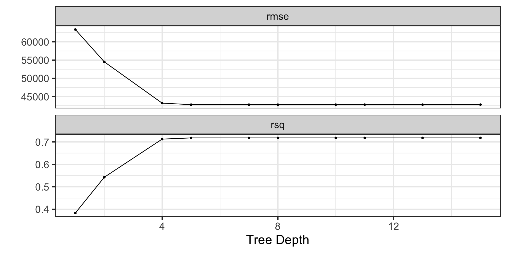
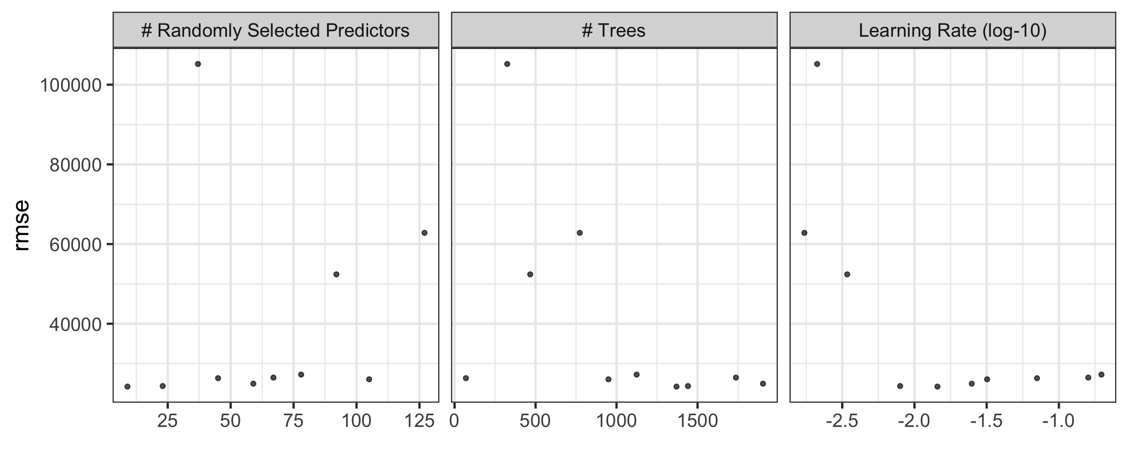
Visualizing the Tuning Results

We see that several tree depths result in models that perform similarly to one another

Eventually, including additional flexibility doesn’t translate into improvements in our model performance metrics

dt_tune_results %>%
  autoplot()

Finalizing the Workflow and Fitting the Best Tree

Now that we’ve obtained our performance metrics and ranked our hyperparameter “combinations”, we can

  1. finalize our workflow with the best parameter choices, and
  2. fit that model to our training data
best_tree <- dt_tune_results %>%
  select_best(metric = "rmse")

dt_wf_final <- dt_wf %>%
  finalize_workflow(best_tree)

dt_fit <- dt_wf_final %>%
  fit(ames_train)

dt_fit
══ Workflow [trained] ══════════════════════════════════════════════════════════
Preprocessor: Recipe
Model: decision_tree()

── Preprocessor ────────────────────────────────────────────────────────────────
2 Recipe Steps

• step_other()
• step_impute_median()

── Model ───────────────────────────────────────────────────────────────────────
n= 2637 

node), split, n, deviance, yval
      * denotes terminal node

 1) root 2637 17265230000000 180593.4  
   2) Garage_Cars< 2.5 2283  6780674000000 160859.2  
     4) Year_Built< 1984.5 1545  3055030000000 140112.9  
       8) Fireplaces< 0.5 907   781422900000 121247.8 *
       9) Fireplaces>=0.5 638  1491915000000 166932.2  
        18) Gr_Liv_Area< 1798.5 489   564099700000 151927.1 *
        19) Gr_Liv_Area>=1798.5 149   456383700000 216177.0 *
     5) Year_Built>=1984.5 738  1668528000000 204291.5  
      10) Total_Bsmt_SF< 1417.5 579   793749400000 191809.7  
        20) Gr_Liv_Area< 1752.5 433   291811200000 177956.7 *
        21) Gr_Liv_Area>=1752.5 146   172403500000 232894.2 *
      11) Total_Bsmt_SF>=1417.5 159   456087700000 249744.2 *
   3) Garage_Cars>=2.5 354  3861633000000 307861.9  
     6) Total_Bsmt_SF< 1721.5 253  1480048000000 271516.1  
      12) Year_Remod_Add< 1977.5 29    40650500000 147827.6 *
      13) Year_Remod_Add>=1977.5 224   938291200000 287529.4  
        26) Gr_Liv_Area< 2322 150   271537500000 259100.1 *
        27) Gr_Liv_Area>=2322 74   299777400000 345156.2 *
     7) Total_Bsmt_SF>=1721.5 101  1210171000000 398906.3  
      14) Gr_Liv_Area< 2217 65   232462900000 353933.4 *
      15) Gr_Liv_Area>=2217 36   608872000000 480107.3 *

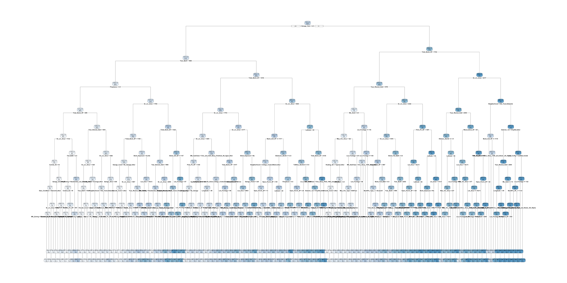
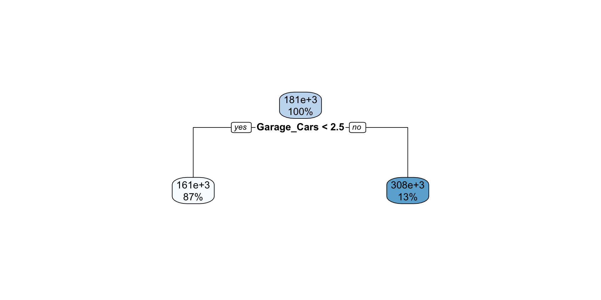
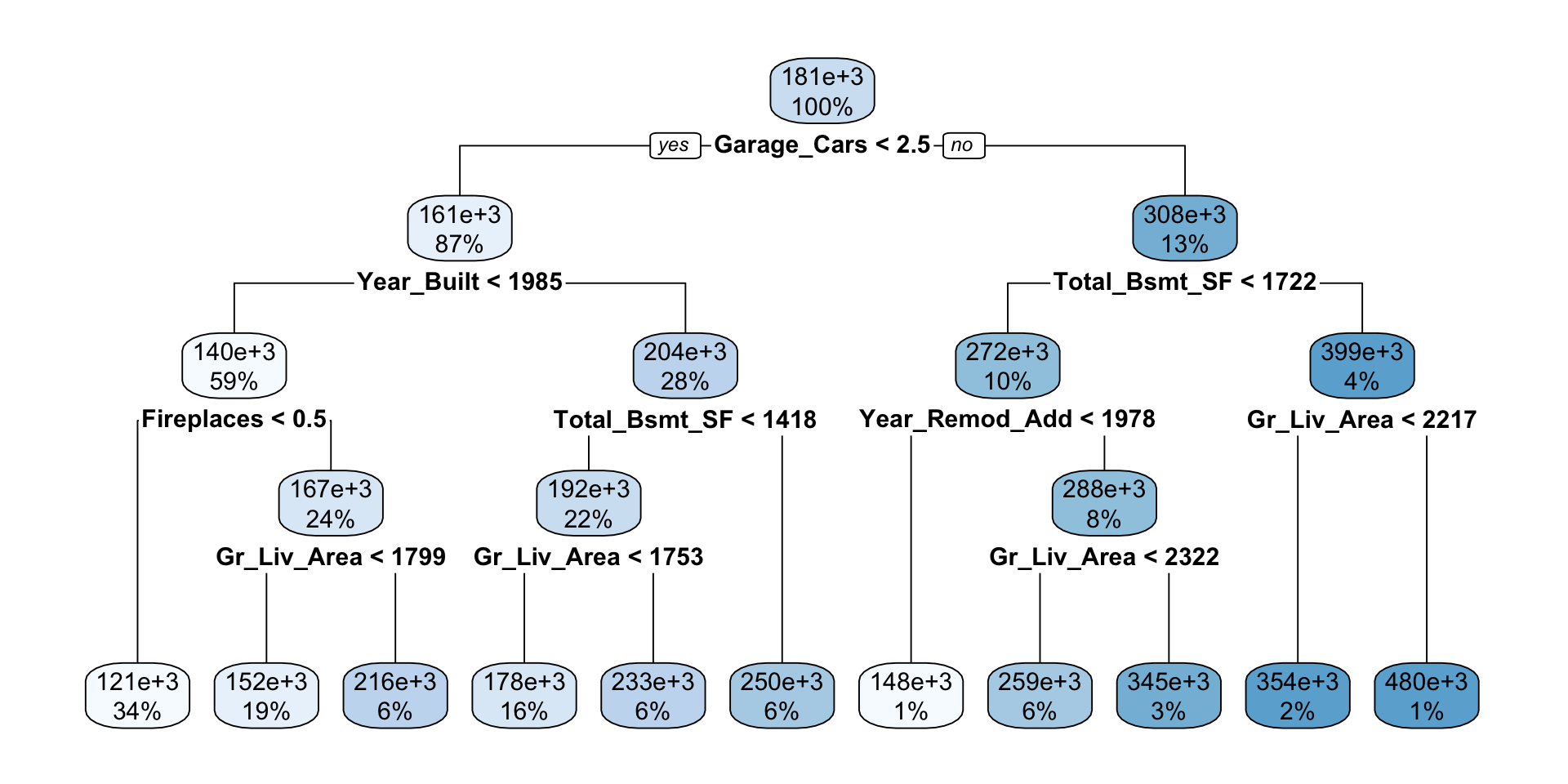
Visualizing the Decision Tree

A major strength of decision trees is how interpretable and intuitive they are (if we can see them)
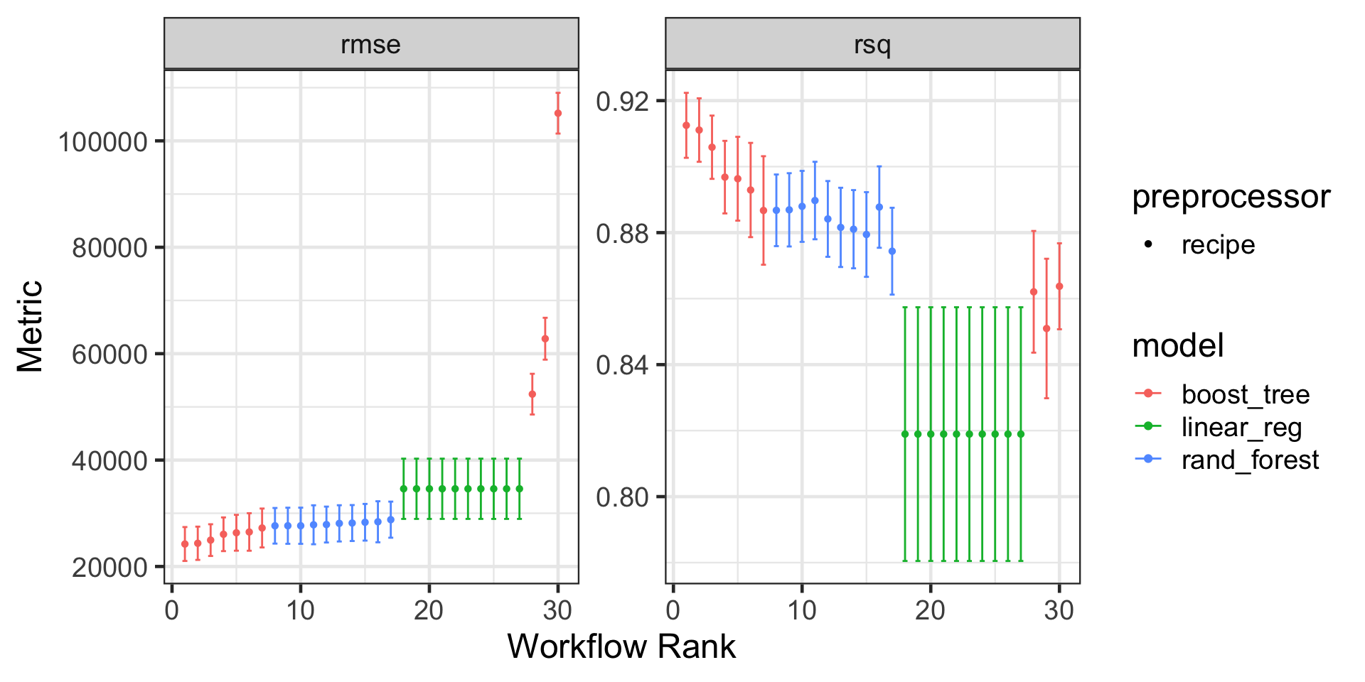
library(rpart.plot)

dt_fit_for_plot <- dt_fit %>%
  extract_fit_engine()

rpart.plot(dt_fit_for_plot)

Crank Up the Tunes!!!

via GIPHY

Tuning Over a Workflow Set

So we’ve got a decision tree model optimized over the tree depth

All we know is that this is the optimal decision tree

What about those other models we talked about??

  • A LASSO?
  • A Random Forest?
  • A Gradient Boosting Ensemble?

Let’s tune all of these models!

Creating the Model Specifications

lasso_spec <- linear_reg(penalty = tune(), mixture = 1) %>%
  set_engine("glmnet")

rf_spec <- rand_forest(mtry = tune(), trees = tune()) %>%
  set_engine("ranger") %>%
  set_mode("regression")

xgb_spec <- boost_tree(mtry = tune(), trees = tune(), learn_rate = tune()) %>%
  set_engine("xgboost") %>%
  set_mode("regression")

A Recipe and Workflow Set

Let’s use the same recipe for all of the models

rec <- recipe(Sale_Price ~ ., data = ames_train) %>%
  step_impute_knn(all_predictors()) %>%
  step_other(all_nominal_predictors()) %>%
  step_dummy(all_nominal_predictors())

Now let’s create the recipe and model lists

rec_list <- list(rec = rec)
model_list <- list(lasso = lasso_spec, rf = rf_spec, xgb = xgb_spec)

And package the lists together into a workflow set

model_wfs <- workflow_set(rec_list, model_list, cross = TRUE)

Constructing a Hyperparameter Grid

We need to define our hyperparameter grid which declares the combinations of hyperparameters we will tune over

param_grid <- grid_regular(
  penalty(),
  mtry(range = c(1, 10)),
  trees(),
  learn_rate(),
  levels = 4
)

Note that we’ve just defined a regular grid of \(4^4 = 256\) hyperparameter combinations

We’re cross-validating our models over five folds and we have three model classes being fit, so now counting model classes, grid combinations, and folds, we have \(3\times 5\times 256 = 3840\) model fits to run

This total ignores that our ensembles consist of 50 - 250 models themselves

Tuning the Models in the Workflow Set

We’ll start by defining the grid controls

grid_ctrl <- control_grid(
  save_pred = TRUE,
  parallel_over = "everything",
  save_workflow = TRUE
)

Using parallel processing will help reduce the time it takes to tune all of our models over all the hyperparameter combinations – let’s tune!

n_cores <- parallel::detectCores()
cluster <- parallel::makeCluster(n_cores - 1, type = "PSOCK")
doParallel::registerDoParallel(cluster)

tictoc::tic()

wfs_tune_results <- model_wfs %>%
  workflow_map(
    seed = 123,
    resamples = ames_folds,
    grid = 10,
    control = grid_ctrl
  )

tictoc::toc()
134.307 sec elapsed

Visualizing Results

wfs_tune_results %>%
  autoplot()

Our Best Model

It looks like the gradient boosting ensemble produced our best results in terms of both RMSE and \(R^2\)

Let’s verify this for RMSE

wfs_tune_results %>% 
  rank_results() %>%
  filter(.metric == "rmse")
wflow_id .config .metric mean std_err n preprocessor model rank
rec_xgb Preprocessor1_Model01 rmse 24224.78 1938.537 5 recipe boost_tree 1
rec_xgb Preprocessor1_Model02 rmse 24363.12 1900.693 5 recipe boost_tree 2
rec_xgb Preprocessor1_Model05 rmse 24956.13 1813.097 5 recipe boost_tree 3
rec_xgb Preprocessor1_Model09 rmse 26054.81 1925.600 5 recipe boost_tree 4
rec_xgb Preprocessor1_Model04 rmse 26337.22 2047.802 5 recipe boost_tree 5
rec_xgb Preprocessor1_Model06 rmse 26486.26 2144.283 5 recipe boost_tree 6
rec_xgb Preprocessor1_Model07 rmse 27236.39 2223.623 5 recipe boost_tree 7
rec_rf Preprocessor1_Model04 rmse 27650.31 2035.178 5 recipe rand_forest 8
rec_rf Preprocessor1_Model06 rmse 27656.36 2063.729 5 recipe rand_forest 9
rec_rf Preprocessor1_Model01 rmse 27657.55 2066.855 5 recipe rand_forest 10

Seeing Best Hyperparameter Combinations

wfs_tune_results %>%
  autoplot(metric = "rmse", id = "rec_xgb")

Extracting Best Hyperparameter Combinations

Let’s extract those best hyperparameter settings

best_model <- wfs_tune_results %>%
  rank_results("rmse", select_best = TRUE) %>%
  head(1) %>%
  pull(wflow_id)

best_wf <- wfs_tune_results %>%
  extract_workflow_set_result(best_model)
  
best_params <- best_wf %>%
  select_best(metric = "rmse")

best_params
mtry trees learn_rate .config
9 1370 0.0144195 Preprocessor1_Model01

Let’s Fit this Best Model

We know our best-performing model was a gradient boosting ensemble, and we’ve stored our optimized hyperparameters in best_params

Let’s construct and fit that model!

best_params <- best_params %>%
  as.list()

set.seed(123)

xgb_spec <- boost_tree(
  trees = best_params$trees,
  mtry = best_params$mtry,
  learn_rate = best_params$learn_rate
) %>%
  set_engine("xgboost") %>%
  set_mode("regression")

xgb_wf <- workflow() %>%
  add_model(xgb_spec) %>%
  add_recipe(rec)

xgb_fit <- xgb_wf %>%
  fit(ames_train)

Extracting Important Predictors

Ensembles are not generally known for their interpretability

We can, however, identify the predictors which are most important to the ensemble using the vip() function from the {vip} package

library(vip)

xgb_fit %>%
  extract_fit_engine() %>%
  vip()

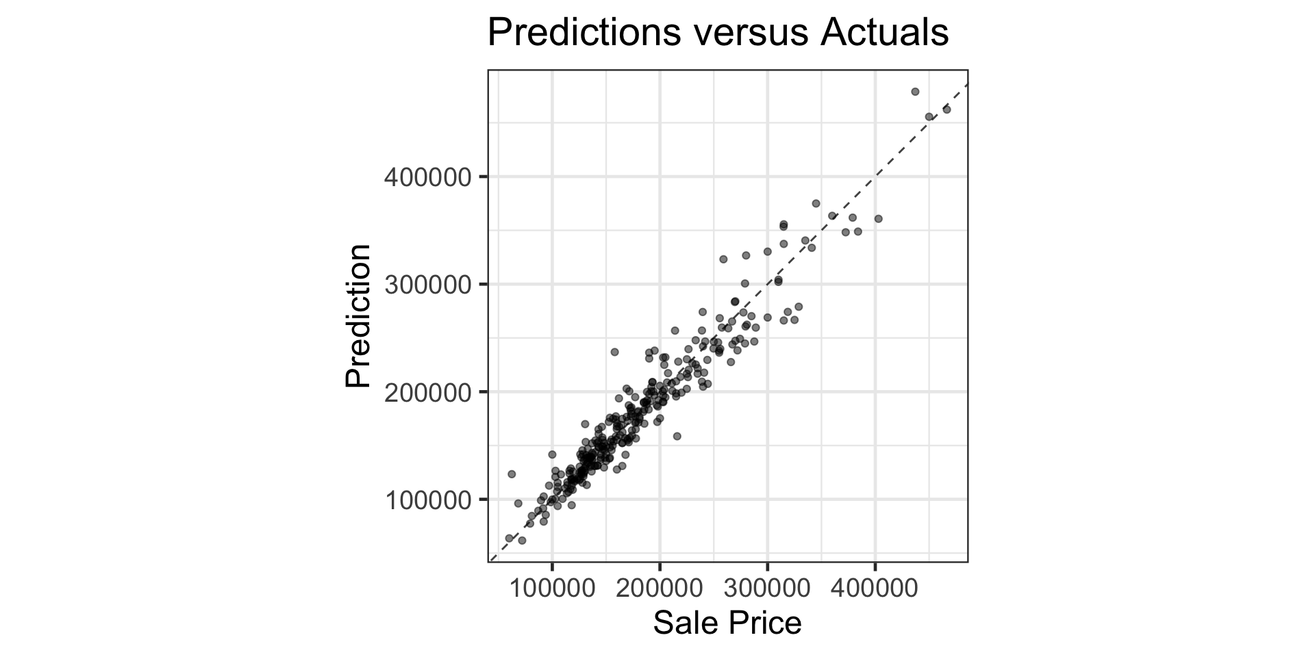
Assessing Performance

Let’s assess our model’s performance on our test data

xgb_results <- xgb_fit %>%
  augment(ames_test) %>%
  select(Sale_Price, .pred)

xgb_results %>%
  ggplot() + 
  geom_point(aes(x = Sale_Price, y = .pred),
             alpha = 0.5) +
  geom_abline(slope = 1, intercept = 0,
              linetype = "dashed", alpha = 0.75) +
  labs(
    title = "Predictions versus Actuals",
    x = "Sale Price",
    y = "Prediction"
  ) + 
  coord_equal()

xgb_results %>%
  rmse(Sale_Price, .pred)
.metric .estimator .estimate
rmse standard 18593.77

Recap

  • We can use cross-validation to tune hyperparameters

    • This means that, after tuning, we can justify our hyperparameter choices
  • We can tune over a workflow set which contains combinations of model specifications and recipes

    • This allows us to not only find an optimal model from a particular class, but an optimal model (including class and hyperpameter settings) from a collection
  • Tuning allows you to improve “off the shelf” models, often by a significant margin

  • Our best untuned model to predict Sale_Price was a Random Forest that had a cross-validation RMSE of $28,606.09, while this tuned gradient boosting ensemble had a cross-validation RMSE of $24,224.78


Go forth and model responsibly!

What’s Next???

Next Time: Hyperparameters, tuning, and other regressors workshop

Then: Thanksgiving In-Class Modeling Competition (there will be prizes, again!)

After That: Final projects for the remainder of the semester

Stop Parallelization

parallel::stopCluster(cluster)