Beyond Linear Regression: Other Classes of Regressor

Dr. Gilbert

September 1, 2024

Recap

We’ve spent the last several weeks investigating and applying linear (and most recently generalized linear) regression models.

\[\mathbb{E}\left[y\right] = \beta_0 + \beta_1 x_1 + \beta_2 x_2 + \cdots + \beta_k x_k\]

We’ve come a long way!

• Simple linear regressors \(\mathbb{E}\left[y\right] = \beta_0 + \beta_1 x\)
• Adding support for multiple numerical predictors
• Allowing for the inclusion of categorical predictors via dummy encodings or scoring
• Accommodating curvature and non-constant associations via higher-order terms
• Using elbow plots to identify appropriate levels of model flexibility
• Using cross-validation to obtain more stable results and more accurate performance estimates
• Engaging in regularization to constrain our models and reduce the likelihood of overfitting

We Did It!

via GIPHY

You should feel accomplished!

We Did It!

via GIPHY

Alternative Regression Models

Regression simply means modeling a numerical response

Linear regression is not the only way to predict a numerical outcome

There are dozens of other model classes suitable for regression problems

• Decision tree regressors
• Nearest neighbor regressors
• Support vector machines
• etc.

We could even utilize an ensemble of models to make predictions – two super common examples are

• Random forests
• Gradient boosting ensembles

Luckily, since the {tidymodels} syntax is standardized, we already know how to fit these models and ensembles!

A Crash Course in Four New Model Classes

KNN Regressors: Nearest neighbor models assume that observations are most like those “closest” to them.

• Identify the “\(k\)” closest training observations to the new observation whose response we want to predict
• Average the responses over those \(k\) neighbors, and that’s the predicted response
• Note: These models are very sensitive to their parameter \(k\)

Decision Tree Regressors: Decision trees mimic human decision-making in an “if this, then that” structure

• Decision trees are very interpretable and easy to explain to non-experts
• Tree-based models are very prone to overfitting, so we must use regularization to constrain them

A Crash Course in Four New Model Classes

An ensemble of models is a collection of models that, together, make a single predicted response

Random Forests: A collection of trees, in parallel, individually making very poor predictions but, when averaged, make an unreasonably accurate prediction

A Crash Course in Four New Model Classes

An ensemble of models is a collection of models that, together, make a single predicted response

Random Forests: A collection of trees, in parallel, individually making very poor predictions but, when averaged, make an unreasonably accurate prediction

• Random forests require each tree to be trained on a slightly different dataset – these are obtained using a procedure called bootstrapping
• For each tree, and at each decision juncture, only a random subset of the predictors are available for the tree to utilize

Gradient Boosting Ensembles: A sequence of very weak (extremely high-bias) learners in series that aim to slowly chip away at the reducible error in predictions

• The first model predicts the response
• The second model predicts the errors made by the first model
• The third model predicts the remaining error made by the first two models, and so on…

Gradient boosting ensembles are very sensitive to the number of boosting rounds and can overfit, if the number of iterations is too high

Five Model Classes, Competing

Let’s try building

• a linear regression model,
• a nearest neighbor regressor,
• a decision tree regressor,
• a random forest, and
• a gradient boosting ensemble of trees

Playing Along

We used the ames data last time and we’ll continue with it today.

1. Open your notebook from last time and run all of the code in it.

2. Add a section on other regression models

Creating Our Model Specifications

Let’s create all five of our model specifications

Several of these models can be used for both regression and classification, so in addition to set_engine(), we’ll also set_mode("regression") for them

lr_spec <- linear_reg() %>%
  set_engine("lm")

dt_spec <- decision_tree(tree_depth = 10, min_n = 3) %>%
  set_engine("rpart") %>%
  set_mode("regression")

knn_spec <- nearest_neighbor(neighbors = 5) %>%
  set_engine("kknn") %>%
  set_mode("regression") 

rf_spec <- rand_forest(mtry = 9, trees = 50, min_n = 3) %>%
  set_engine("ranger") %>%
  set_mode("regression")

xgb_spec <- boost_tree(mtry = 9, trees = 20, tree_depth = 2, learn_rate = 0.1) %>%
  set_engine("xgboost") %>%
  set_mode("regression")

Defining Recipes

Each of these models has different requirements, so we’ll need model-specific recipes

KNN is distance-based, so all predictors should be numeric and scaled

All of the tree-based models (decision tree, random forest, gradient boosting ensemble) can share a recipe

lr_rec <- recipe(Sale_Price ~ ., data = ames_train) %>%
  step_impute_median(all_numeric_predictors()) %>%
  step_other(all_nominal_predictors()) %>%
  step_dummy(all_nominal_predictors())

knn_rec <- recipe(Sale_Price ~ ., data = ames_train) %>%
  step_impute_median(all_numeric_predictors()) %>%
  step_rm(all_nominal_predictors()) %>%
  step_normalize(all_numeric_predictors())

tree_rec <- recipe(Sale_Price ~ ., data = ames_train) %>%
  step_impute_median(all_numeric_predictors()) %>%
  step_other(all_nominal_predictors()) %>%
  step_dummy(all_nominal_predictors())

A Workflow Set

Since we are comparing several models, we can make our lives easier by using a workflow set instead of an individual workflow

Doing this will allow us to cross-validate all of the models at once

We’ll create a list of models, a list of recipes, and then package the lists together into the workflow set

rec_list <- list(
  lr = lr_rec, 
  knn = knn_rec,
  dt = tree_rec,
  rf = tree_rec,
  xgb = tree_rec
)

model_list <- list(
  lr = lr_spec,
  knn = knn_spec,
  dt = dt_spec,
  rf = rf_spec,
  xgb = xgb_spec
)

my_models_wfs <- workflow_set(rec_list, model_list, cross = FALSE)

Fit and Assess the Workflow Set

Now that we’ve got our model specifications and recipes packages into our set of workflows, it’s time to assess them

As you might expect, we’ll use cross-validation for this

Cross-validating over the workflow set is a bit more complicated than cross-validating an individual workflow

grid_ctrl <- control_grid(
  save_pred = TRUE,
  parallel_over = "everything",
  save_workflow = TRUE
)

grid_results <- my_models_wfs %>%
  workflow_map(
    seed = 123,
    resamples = ames_folds,
    control = grid_ctrl)

Okay, So Now What?

Let’s check the results of our cross-validation assessments

grid_results %>%
  autoplot()

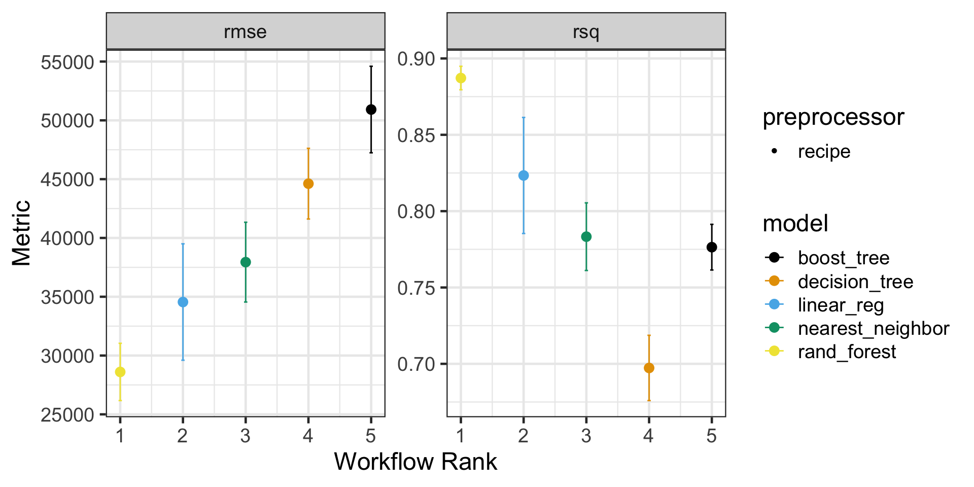
Okay, So Now What?

Let’s check the results of our cross-validation assessments

grid_results %>%
  rank_results()

rank	model	rmse_mean	rmse_se	rsq_mean	rsq_se
1	rand_forest	28606.09	1480.621	0.8871876	0.0046712
2	linear_reg	34551.38	3009.048	0.8233698	0.0231055
3	nearest_neighbor	37943.26	2062.126	0.7832813	0.0134615
4	decision_tree	44615.48	1827.306	0.6973082	0.0129943
5	boost_tree	50919.70	2235.196	0.7764053	0.0090900

I’ve done a bit more to reformat the table than the code I’m showing you will produce

In any case, it looks like our random forest is a pretty clear winner here!

What Now?

Let’s extract that best model from the grid_results

best_results <- grid_results %>%
  extract_workflow_set_result("rf_rf") %>%
  select_best(metric = "rmse")

Now we’ll finalize the workflow for our best (random forest) model-recipe combination, and fit the result to our training/testing split

The result is a fitted model along with predictions for the test observations

rf_test_results <- grid_results %>%
  extract_workflow("rf_rf") %>%
  finalize_workflow(best_results) %>%
  last_fit(split = ames_split)

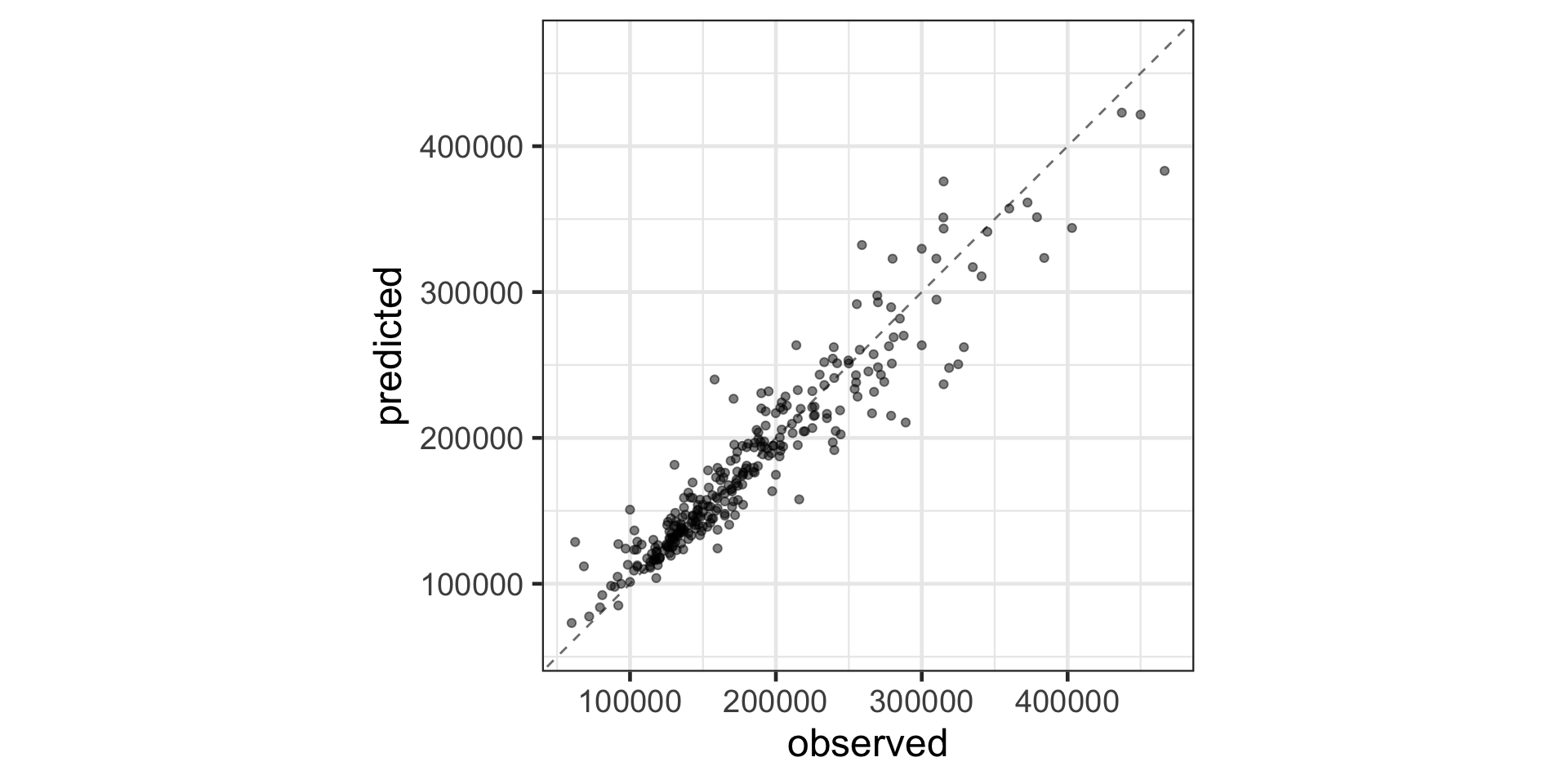
Visualizing Random Forest Performance

Let’s check out how this model does!

rf_test_results %>%
  collect_predictions() %>%
  ggplot() + 
  geom_abline(slope = 1, intercept = 0, color = "gray50", lty = "dashed") +
  geom_point(aes(x = Sale_Price, y = .pred), alpha = 0.5) +
  coord_obs_pred() +
  labs(x = "observed", y = "predicted")

Summary

• There are more model classes available to us than just linear regression
• The {tidymodels} framework provides a streamlined syntax for fitting, assessing, and utilizing lots of the most common types of model (including ensembles)
• We can use our old approaches to define, assess, and compare models one-by-one
• We can also utilize workflow sets to assess multiple model and recipe combinations at once

I hope you’ll explore some of these model classes on your own – especially in our competitions and on your final projects

Next Time…

You may have noticed that, ever since we discussed regularization methods, we’ve been setting parameters prior to our models seeing any data

• mixture
• penalty
• mtry
• trees
• neighbors
• etc.

How do we know that we’ve chosen the best values?

How do we even know that we’ve chosen appropriate values?

Hyperparameter Tuning