Hyperparameters and Model Tuning

Published

August 3, 2024

Code
#install.packages("xgboost")
library(tidyverse)
library(tidymodels)
library(patchwork)
library(kableExtra)
library(modeldata)

tidymodels_prefer()

options(kable_styling_bootstrap_options = c("hover", "striped"))

#Set ggplot base theme
theme_set(theme_bw(base_size = 14))

ames <- read_csv("https://raw.githubusercontent.com/koalaverse/homlr/master/data/ames.csv")

Recap

In our most recent notebooks, we’ve gone beyond Ordinary Least Squares and explored additional classes of model. We began with penalized least squares models like Ridge Regression and the LASSO. We extended our knowledge of model classes to nearest neighbor and tree-based models as well as ensembles of models in the previous notebook. We ended that notebook with a short discussion on parameter choices that must be made prior to model training – such parameters are known as hyperparameters. In this notebook, we learn how to use cross-validation to tune our model hyperparameters.

Objectives

In this notebook, we’ll accomplish the following:

  • Use tune() for model parameters as well as in feature engineering steps to identify hyperparameters that we want to tune through cross-validation.
  • Use cross-validation and tune_grid() to tune the hyperparameters for a single model, identify the best hyperparameter choices, and fit the model using those best choices.
  • Build a workflow_set(), choose hyperparameters that must be tuned for each model and recipe, use cross-validation to tune models and select “optimal” hyperparameter values, and compare the models in the workflow set.

Tuning Hyperparameters for a Single Model

Let’s start with a decision tree model and we’ll tune the tree depth parameter. We’ll work with the ames data again for now.

ames_known_prices <- ames %>%
  filter(!is.na(Sale_Price))

ames_split <- initial_split(ames_known_prices, prop = 0.9)
ames_train <- training(ames_split)
ames_test <- testing(ames_split)

ames_folds <- vfold_cv(ames_train, v = 5)

tree_spec <- decision_tree(tree_depth = tune()) %>%
  set_engine("rpart") %>%
  set_mode("regression")

tree_rec <- recipe(Sale_Price ~ ., data = ames_train) %>%
  step_other(all_nominal_predictors()) %>%
  step_unknown(all_nominal_predictors()) %>%
  step_impute_median(all_numeric_predictors())

tree_wf <- workflow() %>%
  add_model(tree_spec) %>%
  add_recipe(tree_rec)

set.seed(123)
tree_results <- tree_wf %>%
  tune_grid(ames_folds, grid =12)

tree_results %>%
  autoplot()

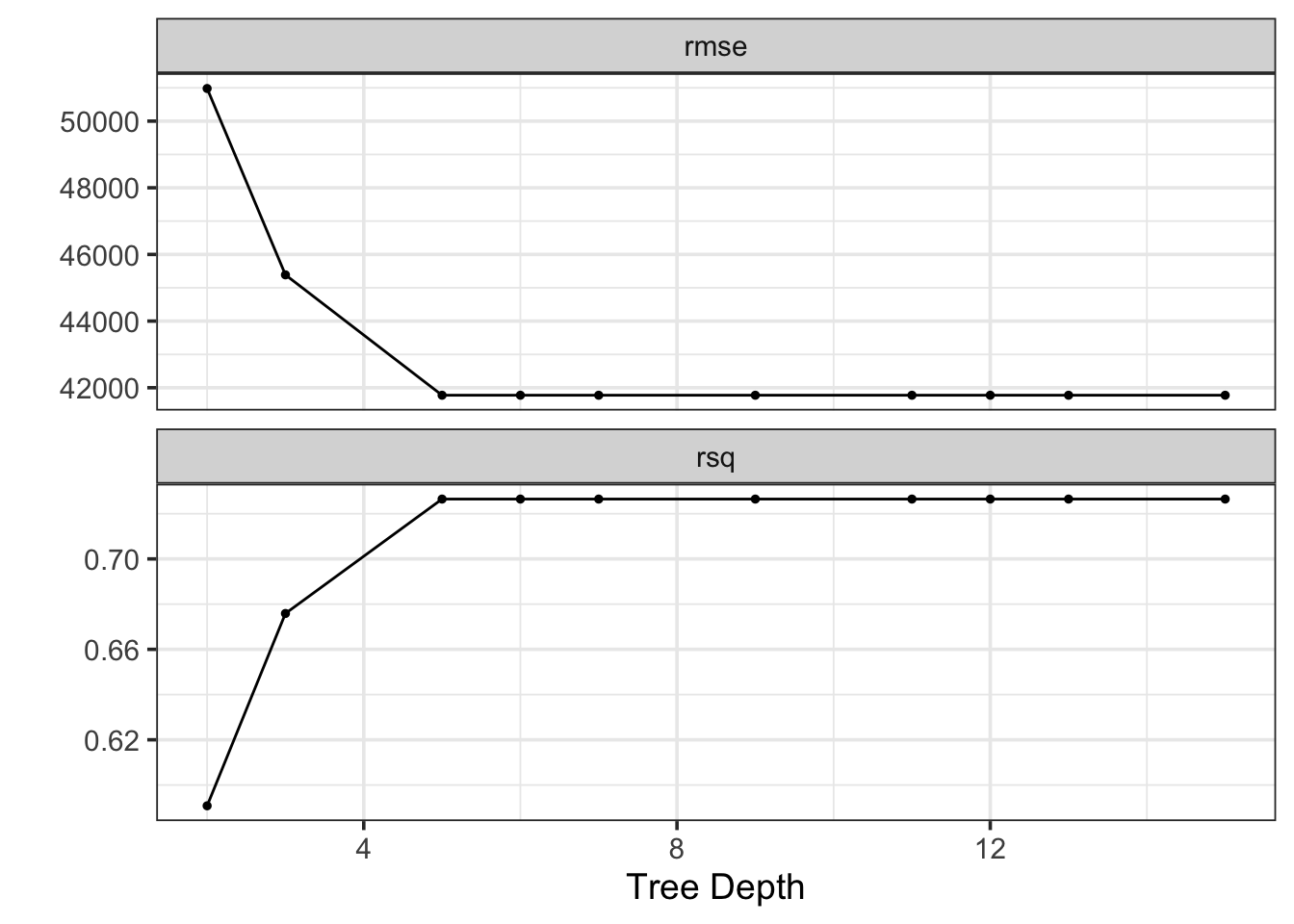
We see from the plots above that deeper trees seemed to perform better than shallow trees. We don’t observe much improvement in performance after a depth of 5. The risk of overfitting increases with deeper trees. We do seem to get some benefit by increasing the depth of the tree beyond 4. For this reason, I’ll choose a tree depth of 5. The output of show_best() below shows our best-performing depths in terms of RMSE.

tree_results %>%
  show_best(n = 10) %>%
  kable() %>%
  kable_styling()
Warning in show_best(., n = 10): No value of `metric` was given; "rmse" will be
used.
tree_depth .metric .estimator mean n std_err .config
12 rmse standard 41775.44 5 704.2423 Preprocessor1_Model01
7 rmse standard 41775.44 5 704.2423 Preprocessor1_Model02
9 rmse standard 41775.44 5 704.2423 Preprocessor1_Model03
11 rmse standard 41775.44 5 704.2423 Preprocessor1_Model05
6 rmse standard 41775.44 5 704.2423 Preprocessor1_Model06
15 rmse standard 41775.44 5 704.2423 Preprocessor1_Model07
5 rmse standard 41775.44 5 704.2423 Preprocessor1_Model08
13 rmse standard 41775.44 5 704.2423 Preprocessor1_Model10
3 rmse standard 45387.60 5 1158.2563 Preprocessor1_Model04
2 rmse standard 50978.88 5 1129.1382 Preprocessor1_Model09

We can now build a final fit using this depth.

best_params <- tibble(tree_depth = 5)

tree_wf_final <- tree_wf %>%
  finalize_workflow(best_params)

tree_fit <- tree_wf_final %>%
  fit(ames_train)

tree_fit
══ Workflow [trained] ══════════════════════════════════════════════════════════
Preprocessor: Recipe
Model: decision_tree()

── Preprocessor ────────────────────────────────────────────────────────────────
3 Recipe Steps

• step_other()
• step_unknown()
• step_impute_median()

── Model ───────────────────────────────────────────────────────────────────────
n= 2637 

node), split, n, deviance, yval
      * denotes terminal node

 1) root 2637 1.667211e+13 180558.00  
   2) Garage_Cars< 2.5 2285 6.690571e+12 161328.70  
     4) Overall_Qual=Above_Average,Average,Below_Average,other 1640 2.917557e+12 141681.30  
       8) Gr_Liv_Area< 1376.5 1005 8.828377e+11 125065.70  
        16) Overall_Qual=Below_Average,other 192 1.774146e+11  93651.44 *
        17) Overall_Qual=Above_Average,Average 813 4.711992e+11 132484.60 *
       9) Gr_Liv_Area>=1376.5 635 1.318134e+12 167978.40  
        18) Kitchen_Qual=Typical,other 436 4.940404e+11 154393.50 *
        19) Kitchen_Qual=Excellent,Good 199 5.673376e+11 197742.40  
          38) Overall_Qual=Above_Average,Average,Below_Average 179 3.099228e+11 186715.90 *
          39) Overall_Qual=other 20 4.086997e+10 296429.20 *
     5) Overall_Qual=Good,Very_Good 645 1.530270e+12 211284.80  
      10) First_Flr_SF< 1493 510 8.232808e+11 199269.20  
        20) Gr_Liv_Area< 1779.5 355 3.616527e+11 185992.10 *
        21) Gr_Liv_Area>=1779.5 155 2.557208e+11 229678.00 *
      11) First_Flr_SF>=1493 135 3.551916e+11 256677.40 *
   3) Garage_Cars>=2.5 352 3.651879e+12 305384.50  
     6) Kitchen_Qual=Good,Typical 233 1.258540e+12 262063.60  
      12) Year_Remod_Add< 1979 32 4.427554e+10 148371.90 *
      13) Year_Remod_Add>=1979 201 7.347876e+11 280163.80  
        26) Gr_Liv_Area< 1963 116 2.461216e+11 252483.00 *
        27) Gr_Liv_Area>=1963 85 2.784864e+11 317939.80 *
     7) Kitchen_Qual=Excellent 119 1.099895e+12 390206.30  
      14) Gr_Liv_Area< 2220 63 1.663214e+11 344960.40 *
      15) Gr_Liv_Area>=2220 56 6.595061e+11 441107.80 *

We can see the tree as well, using rpart.plot().

library(rpart.plot)

tree_fit_for_plot <- tree_fit %>%
  extract_fit_engine()

rpart.plot(tree_fit_for_plot, tweak = 1.5)
Warning: Cannot retrieve the data used to build the model (so cannot determine roundint and is.binary for the variables).
To silence this warning:
    Call rpart.plot with roundint=FALSE,
    or rebuild the rpart model with model=TRUE.

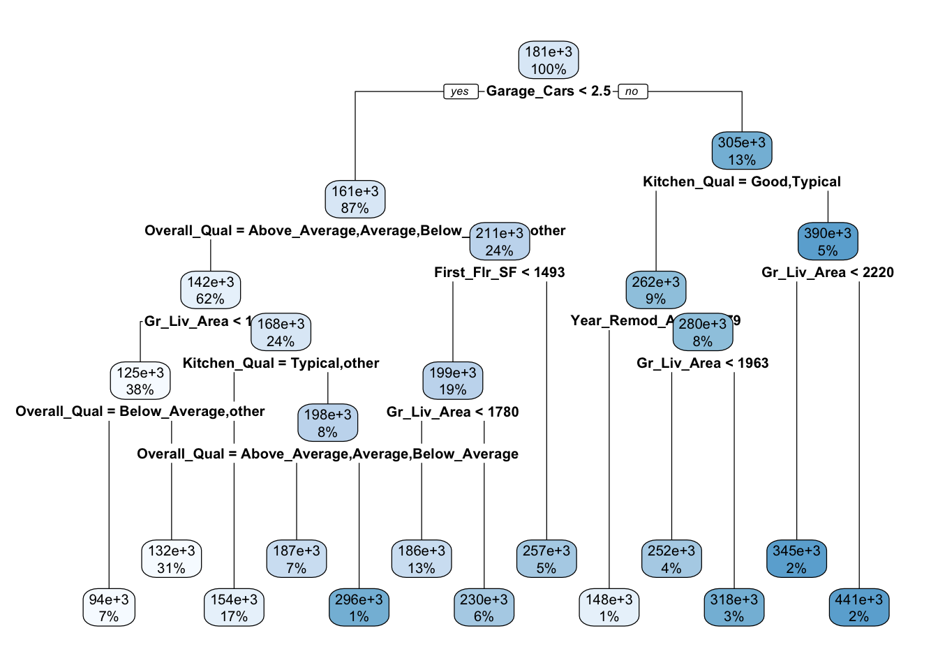
The model we built above can be interpreted and can also be utilized to make predictions on new data just like out previous models. Next, let’s look at how we can tune multiple models with a variety of hyperparameters in a workflow_set(). We’ll fit a LASSO, a random forest, and a gradient boosted model.

Tuning Hyperparameters Across a Workflow Set

Let’s create model specifications and recipes for each of the models mentioned in earlier notebooks.

doParallel::registerDoParallel()

lasso_spec <- linear_reg(penalty = tune(), mixture = 1) %>%
  set_engine("glmnet")

rf_spec <- rand_forest(mtry = tune(), trees = 100) %>%
  set_engine("ranger") %>%
  set_mode("regression")

gb_spec <- boost_tree(mtry = tune(), trees = 100, learn_rate = tune()) %>%
  set_engine("xgboost") %>%
  set_mode("regression")
  
rec <- recipe(Sale_Price ~ ., data = ames_train) %>%
  step_impute_knn(all_predictors()) %>%
  step_other(all_nominal_predictors(), threshold = 0.10) %>%
  step_dummy(all_nominal_predictors())

rec_list = list(rec = rec)
model_list = list(lasso = lasso_spec, rf = rf_spec, gb_tree = gb_spec)

model_wfs <- workflow_set(rec_list, model_list, cross = TRUE)

grid_ctrl <- control_grid(
  save_pred = TRUE,
  parallel_over = "everything",
  save_workflow = TRUE
)

grid_results <- model_wfs %>%
  workflow_map(
    seed = 123,
    resamples = ames_folds,
    grid = 5,
    control = grid_ctrl)
i Creating pre-processing data to finalize unknown parameter: mtry
grid_results %>%
  autoplot()

Now let’s see what the best models were!

grid_results %>%
  rank_results() %>%
  kable() %>%
  kable_styling()
wflow_id .config .metric mean std_err n preprocessor model rank
rec_gb_tree Preprocessor1_Model2 rmse 2.405655e+04 782.1749664 5 recipe boost_tree 1
rec_gb_tree Preprocessor1_Model2 rsq 9.092399e-01 0.0054418 5 recipe boost_tree 1
rec_gb_tree Preprocessor1_Model3 rmse 2.460431e+04 1185.2240259 5 recipe boost_tree 2
rec_gb_tree Preprocessor1_Model3 rsq 9.057068e-01 0.0092678 5 recipe boost_tree 2
rec_rf Preprocessor1_Model3 rmse 2.649436e+04 751.2181872 5 recipe rand_forest 3
rec_rf Preprocessor1_Model3 rsq 8.922140e-01 0.0039914 5 recipe rand_forest 3
rec_rf Preprocessor1_Model5 rmse 2.667734e+04 880.1102319 5 recipe rand_forest 4
rec_rf Preprocessor1_Model5 rsq 8.914213e-01 0.0067577 5 recipe rand_forest 4
rec_rf Preprocessor1_Model1 rmse 2.681196e+04 776.3474654 5 recipe rand_forest 5
rec_rf Preprocessor1_Model1 rsq 8.896710e-01 0.0055748 5 recipe rand_forest 5
rec_rf Preprocessor1_Model2 rmse 2.702251e+04 727.9304682 5 recipe rand_forest 6
rec_rf Preprocessor1_Model2 rsq 8.876737e-01 0.0053559 5 recipe rand_forest 6
rec_lasso Preprocessor1_Model5 rmse 3.463037e+04 2726.0237672 5 recipe linear_reg 7
rec_lasso Preprocessor1_Model5 rsq 8.178759e-01 0.0241675 5 recipe linear_reg 7
rec_lasso Preprocessor1_Model1 rmse 3.463037e+04 2726.0237672 5 recipe linear_reg 8
rec_lasso Preprocessor1_Model1 rsq 8.178759e-01 0.0241675 5 recipe linear_reg 8
rec_lasso Preprocessor1_Model2 rmse 3.463037e+04 2726.0237672 5 recipe linear_reg 9
rec_lasso Preprocessor1_Model2 rsq 8.178759e-01 0.0241675 5 recipe linear_reg 9
rec_lasso Preprocessor1_Model3 rmse 3.463037e+04 2726.0237672 5 recipe linear_reg 10
rec_lasso Preprocessor1_Model3 rsq 8.178759e-01 0.0241675 5 recipe linear_reg 10
rec_lasso Preprocessor1_Model4 rmse 3.463037e+04 2726.0237672 5 recipe linear_reg 11
rec_lasso Preprocessor1_Model4 rsq 8.178759e-01 0.0241675 5 recipe linear_reg 11
rec_gb_tree Preprocessor1_Model1 rmse 3.984044e+04 1111.5806383 5 recipe boost_tree 12
rec_gb_tree Preprocessor1_Model1 rsq 8.865721e-01 0.0067209 5 recipe boost_tree 12
rec_rf Preprocessor1_Model4 rmse 4.678976e+04 1368.0043202 5 recipe rand_forest 13
rec_rf Preprocessor1_Model4 rsq 8.019057e-01 0.0073440 5 recipe rand_forest 13
rec_gb_tree Preprocessor1_Model5 rmse 9.912738e+04 945.9103046 5 recipe boost_tree 14
rec_gb_tree Preprocessor1_Model5 rsq 8.504925e-01 0.0081082 5 recipe boost_tree 14
rec_gb_tree Preprocessor1_Model4 rmse 1.654890e+05 1168.5860783 5 recipe boost_tree 15
rec_gb_tree Preprocessor1_Model4 rsq 8.555862e-01 0.0076431 5 recipe boost_tree 15

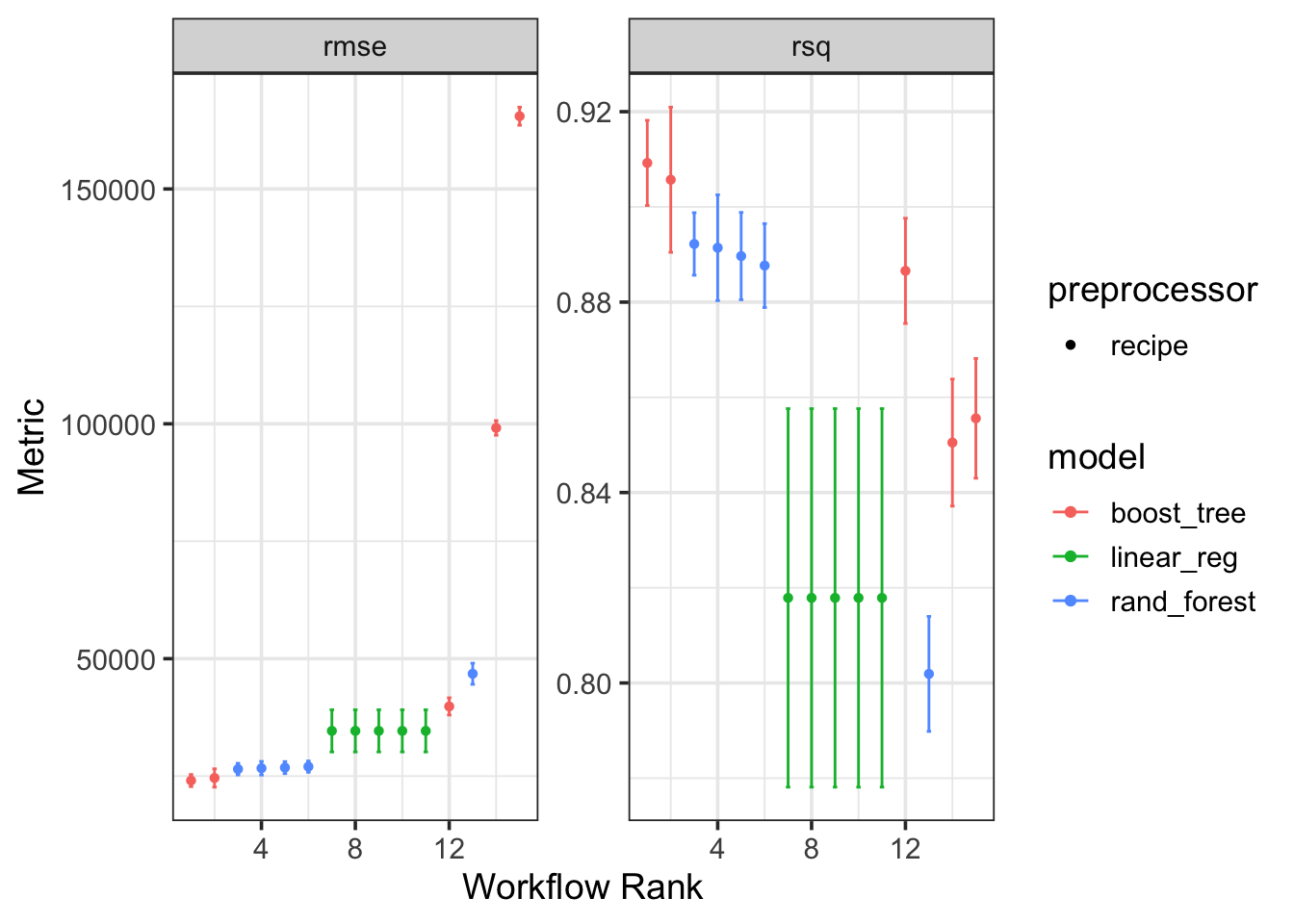
The model performing the best was the gradient boosted tree ensemble. Let’s see what hyperparameter choices led to the best performance.
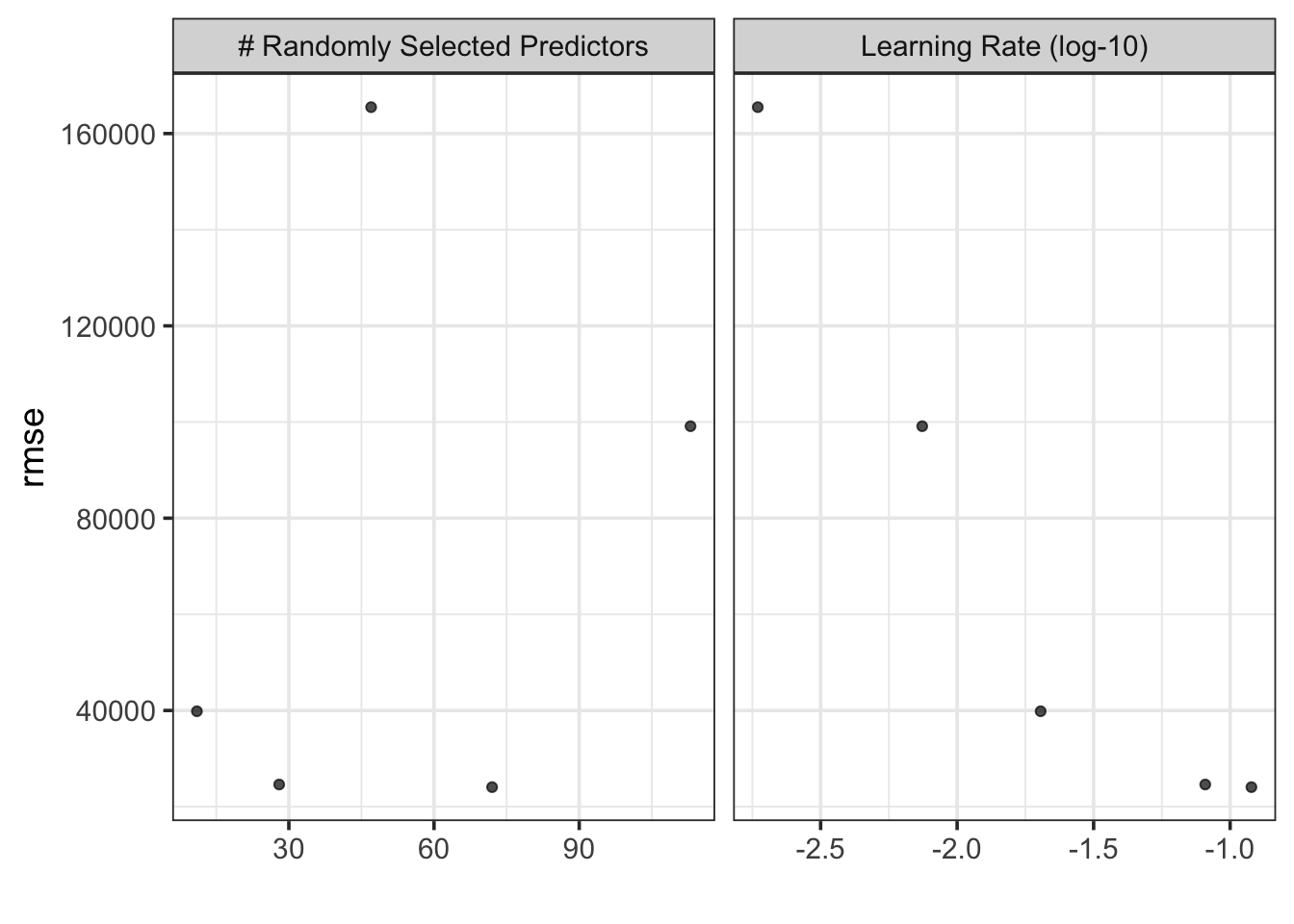
grid_results %>%
  autoplot(metric = "rmse", id = "rec_gb_tree")

It seems that a number of randomly selected parameters of near 30 gave the best performance and learning rates near 0.1 did as well. We’ll construct this model and fit it to our training data.

set.seed(123)
gb_tree_spec <- boost_tree(mtry = 30, trees = 100, learn_rate = 0.1) %>%
  set_engine("xgboost") %>%
  set_mode("regression")

gb_tree_wf <- workflow() %>%
  add_model(gb_tree_spec) %>%
  add_recipe(rec)

gb_tree_fit <- gb_tree_wf %>%
  fit(ames_train)

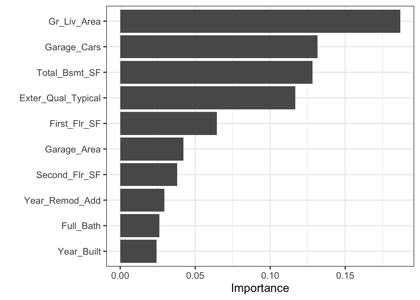
Such a model doesn’t have much interpretive value but can make very good predictions. We can identify the predictors which were most important within the ensemble by using var_imp().

library(vip)
gb_tree_fit %>%
  extract_fit_engine() %>%
  vip()

From the plot above, we can see the features that were most the important predictors of selling price within the ensemble. Note that the important predictors will shuffle around slightly each time you re-run the ensemble. Before we close this notebook, let’s take a look at how well this model predicts the selling prices of homes in our test set.

gb_results <- gb_tree_fit %>%
  augment(ames_test) %>%
  select(Sale_Price, .pred) %>%
  rmse(Sale_Price, .pred) 

gb_results %>%
  kable() %>%
  kable_styling(bootstrap_options = c("striped", "hover"))
.metric .estimator .estimate
rmse standard 20582.85

This final ensemble of models predicted selling prices of homes with an root mean squared error of $ 20,582.85.

Summary

In this notebook, we saw how to build a workflow set consisting of several models with tunable hyperparameters. We explored a space-filling grid of hyperparameter combinations with a workflow_map(). After identifying a best model and optimal(*) hyperparameter choices, we fit the corresponding model to our training data and then assessed that model’s performance on our test data.