The Bias/Variance TradeOff

Dr. Gilbert

September 1, 2024

Motivation

Recap

We’ve been hypothesizing, building, assessing, and interpreting regression models

\[\mathbb{E}\left[y\right] = \beta_0 + \beta_1 x_1 + \beta_2 x_2 + \cdots + \beta_k x_k\]

for the past few weeks

• We began with simple linear regression and multiple linear regression, where the predictors \(x_1, \cdots, x_k\) were independent, numerical predictors.

  • We interpreted each \(\beta_i\) (other than \(\beta_0\)) as the expected change in the response given a unit increase in the corresponding predictor \(x_i\) – (\(\beta_i\) was a slope)

• We considered strategies for adding categorical predictors to our models

  • We used dummy variables which could take values of 0 or 1 – each \(\beta_i\) corresponding to a dummy variable was an intercept adjustment

• We expanded our ability to fit complex relationships by considering higher-order terms

  • Polynomial terms accommodated curvature in the relationship between a numerical predictor and the response
  • Interaction terms allowed for the association between a predictor and the response to depend on the level of another predictor

Recap

Each time we expanded our modeling abilities, we introduced additional \(\beta\)-parameters to our models

This gave us several advantages:

• Improved fit to our training data
• Greater ability to model, discover, and explain complex relationships

And some disadvantages:

• More data required to fit these models
• More difficulty in interpreting models

There’s a question we’ve been neglecting though…

Does improved fit to our training data actually translate to a better (more accurate, more meaningful) model in practice?

The Big Concern and Questions

Increasing the number of \(\beta\)-parameters in a model (by including dummy variables, higher-order terms, etc.) increases the flexibility of our model

This means that our model can accommodate more complex relationships – whether they are signal or noise

This also means that our model becomes more sensitive to its training data

1. More \(\beta\) coefficients means better training performance (higher \(R^2\), lower RMSE, etc.) in general

2. The more \(\beta\) coefficients we have, the greater the likelihood that we are overfitting to our training data

Question 1: If all those great strategies we’ve learned recently are increasing our risk of overfitting, should we really be using them?

Question 2: How do we know whether we are overfitting or not?

Question 3: Can we know?

Highlights

We’ll look at the following items as we try to answer those three questions.

• What are bias and variance?
• How do bias and variance manifest themselves in our models?
• How are bias and variance connected to model flexibility?
• How are bias, variance, and model flexibility connected to overfitting and underfitting?
• Training error, test error, and identifying appropriate model flexibility to solve the bias/variance trade-off problem

Bias and Variance

The level of bias in a model is a measure of how conservative that model is

• Models with high bias have low flexibility – they are more rigid/straight/flat
• Models with low bias have high flexibility – they can wiggle around a lot, allowing them to get closer to more training observations

The level of variance in a model is a measure of how much that model would change, given different training data from the same population

• Models with low variance change little even if given slightly different training data
• Models with high variance may change wildly under a slightly different training set

Seeing Bias and Variance in Models

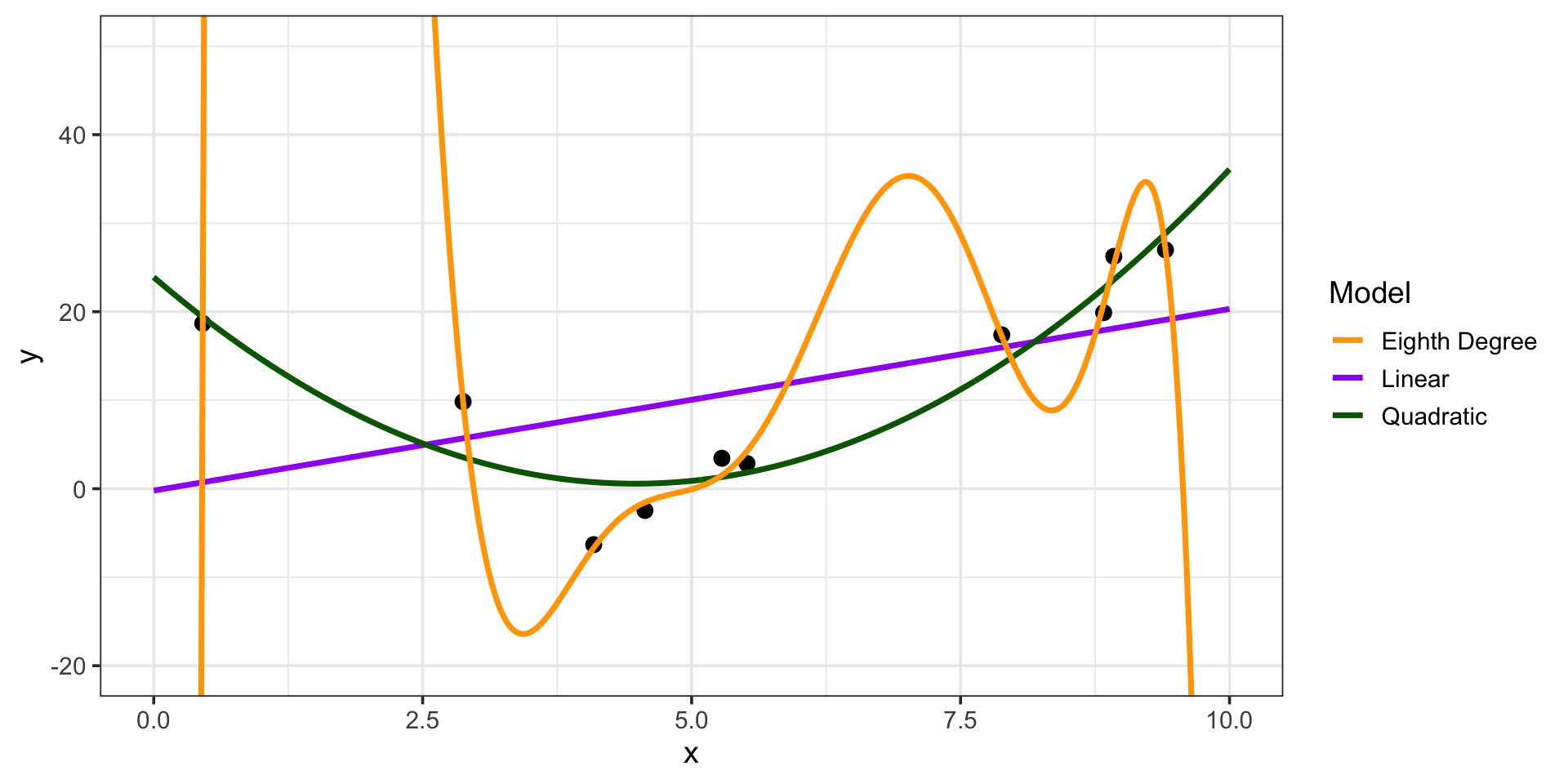
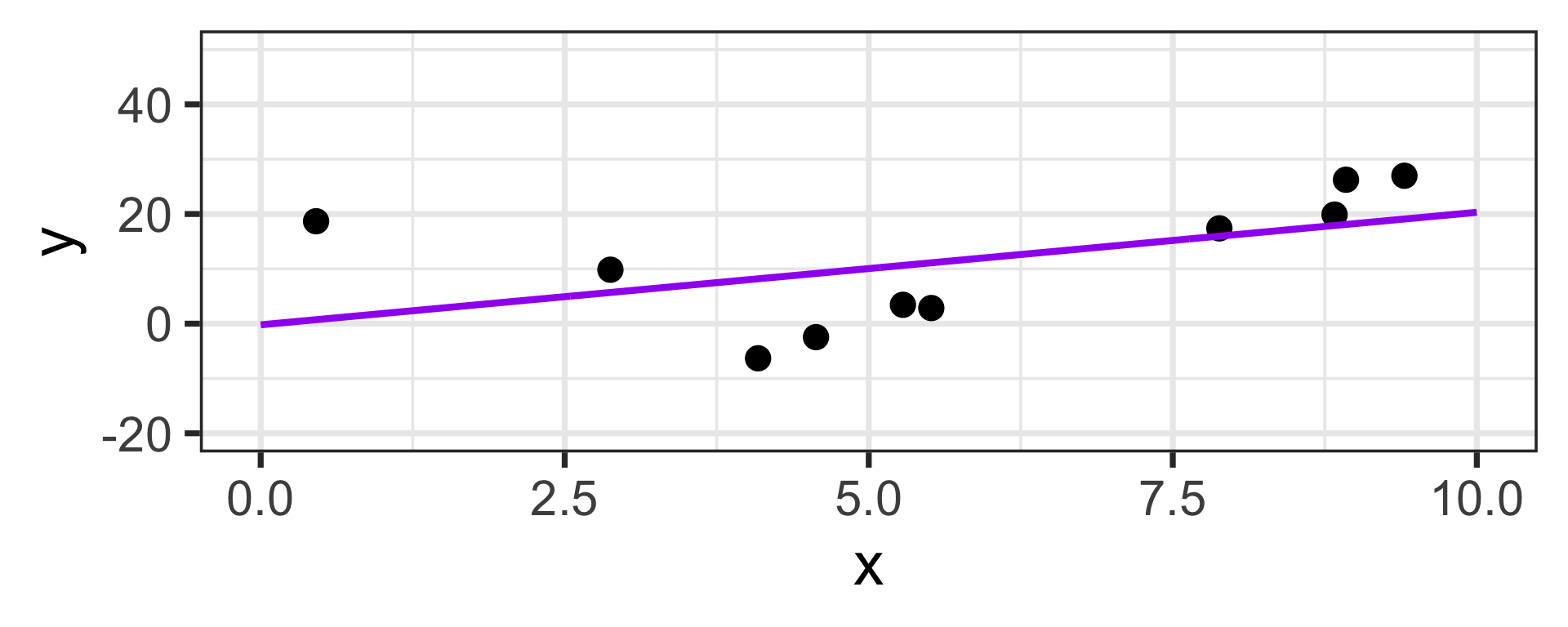
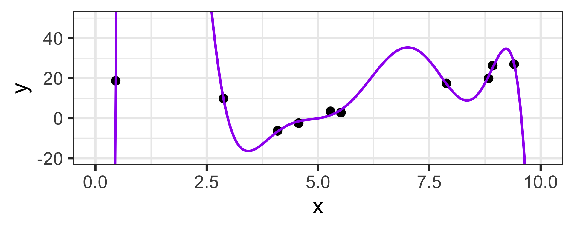
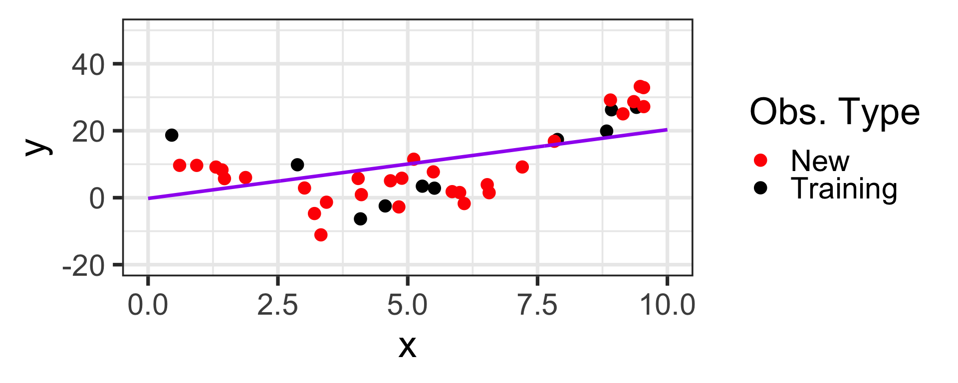
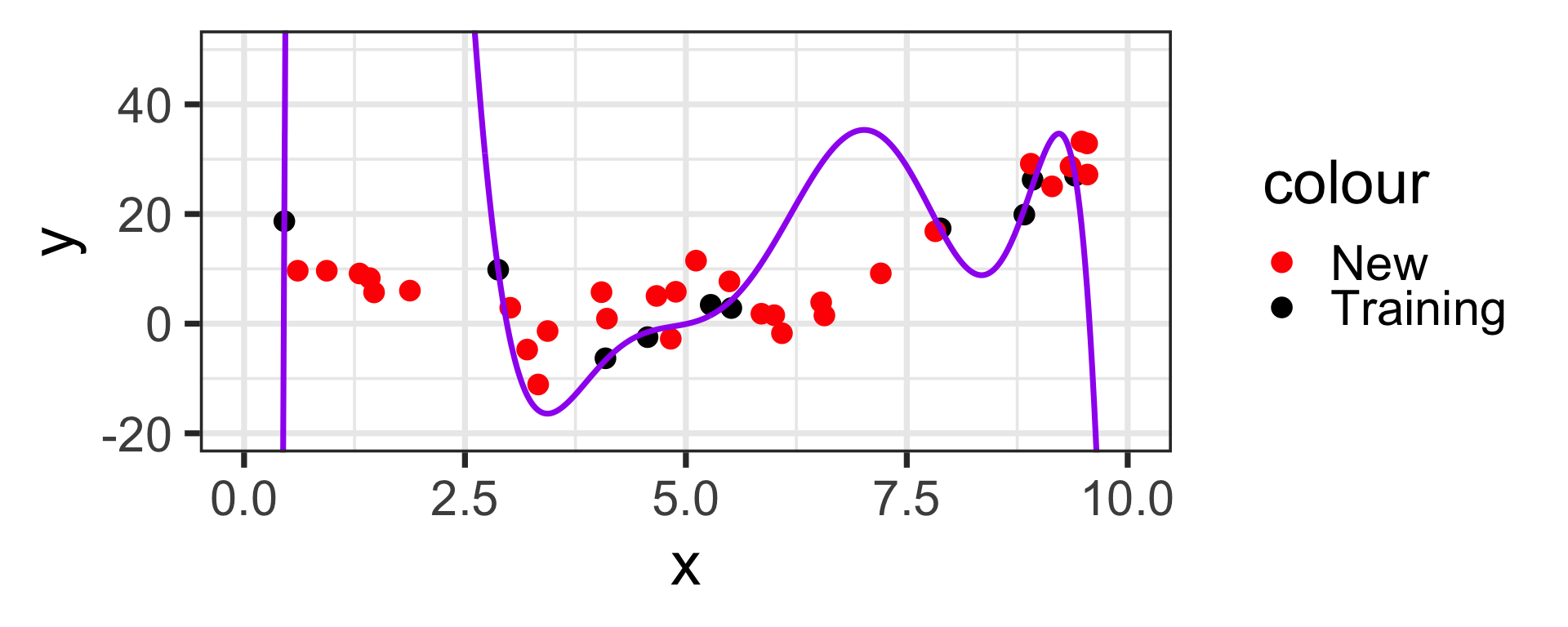
Let’s bring back our Linear and Eighth Degree models from the opening slide

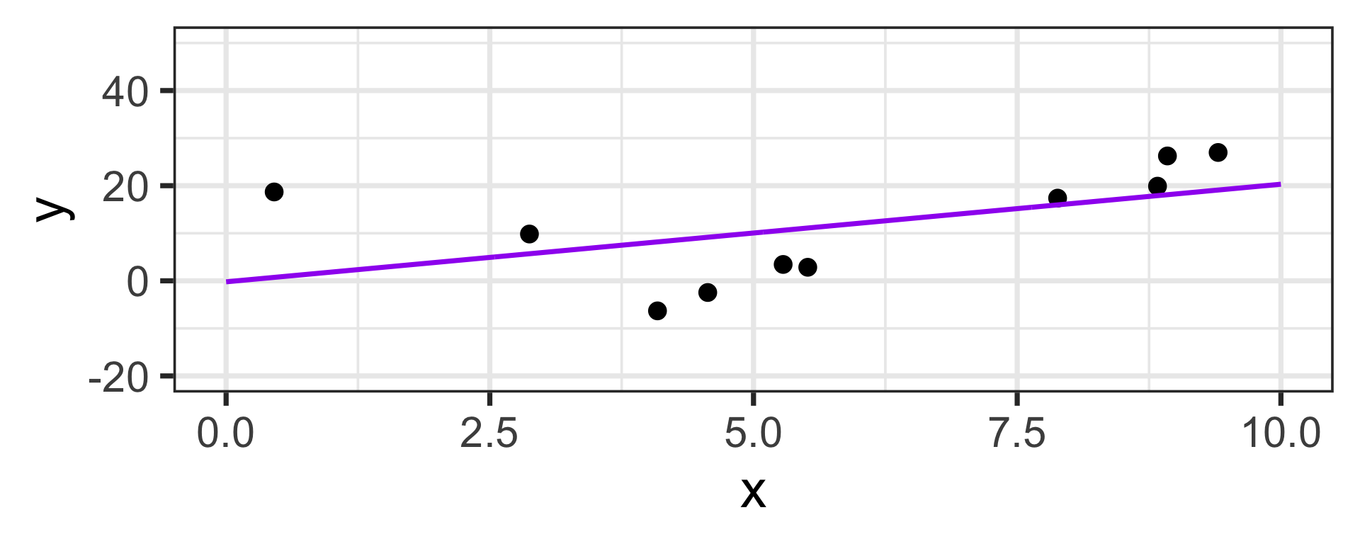
High Bias / Low Variance:

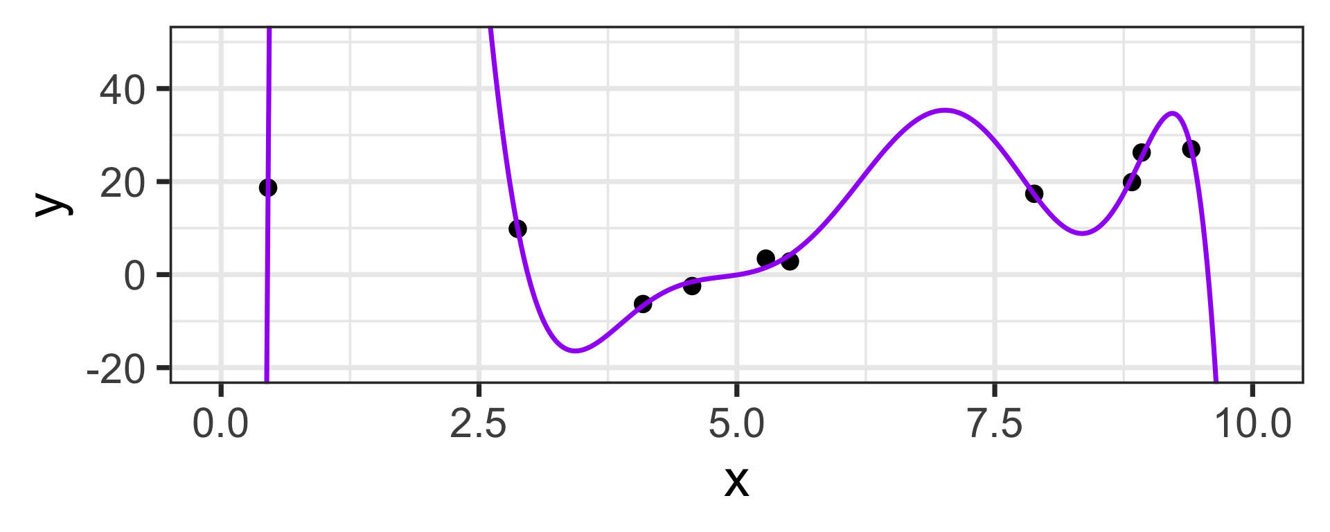
Low Bias / High Variance:

Let’s consider what would happen if we had a new training observation at \(x = 7\), \(y = 5\)

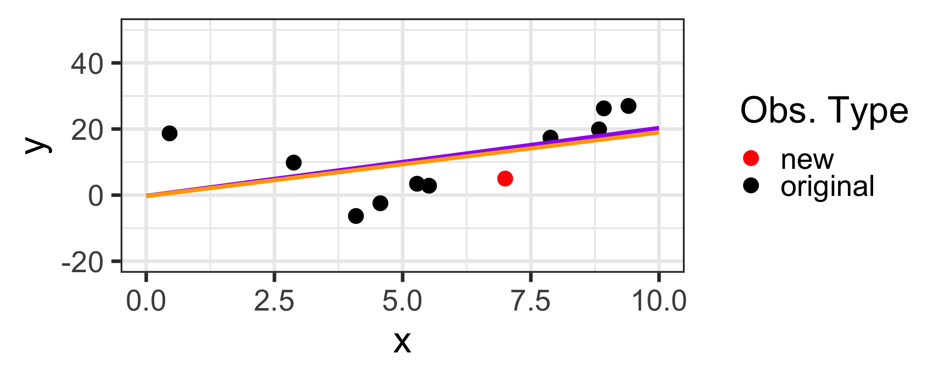
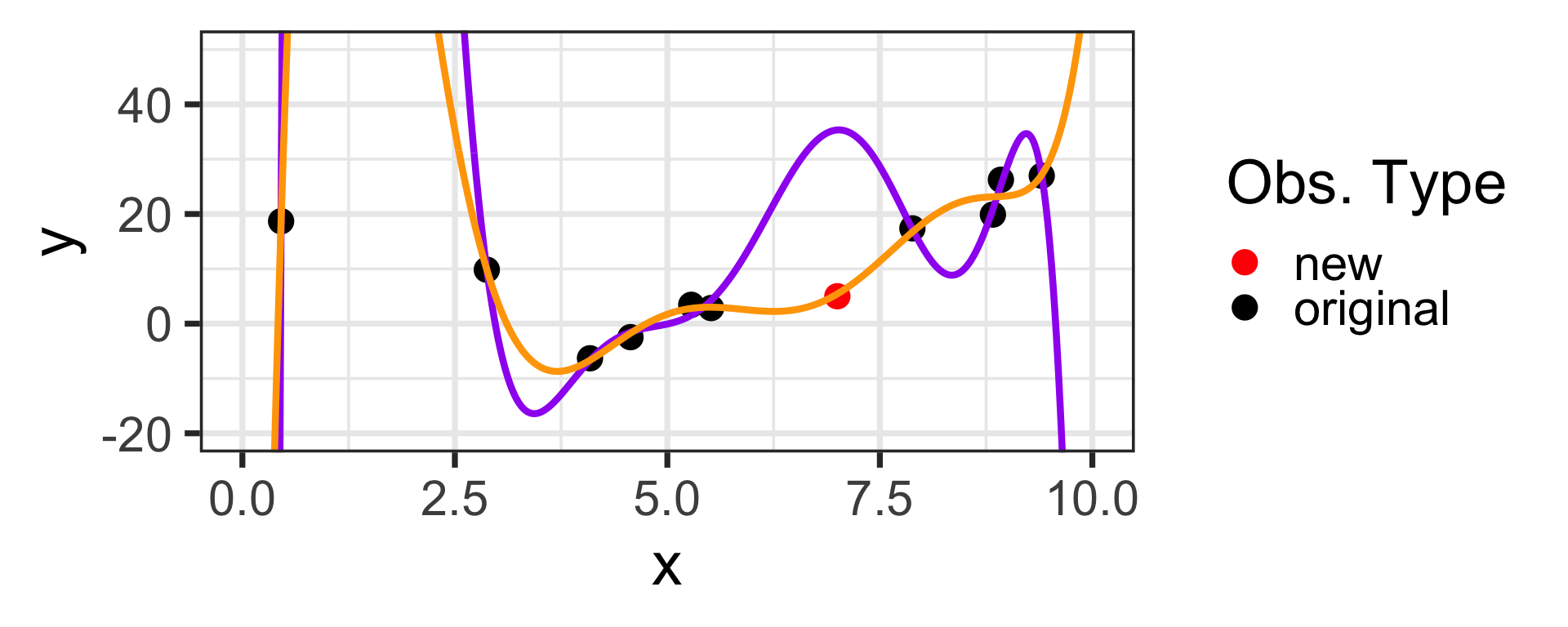
Oh No!

Seeing Bias in Our Models

On the previous slide, we saw very clearly that the model on the right had bias which was too low and variance that was too high

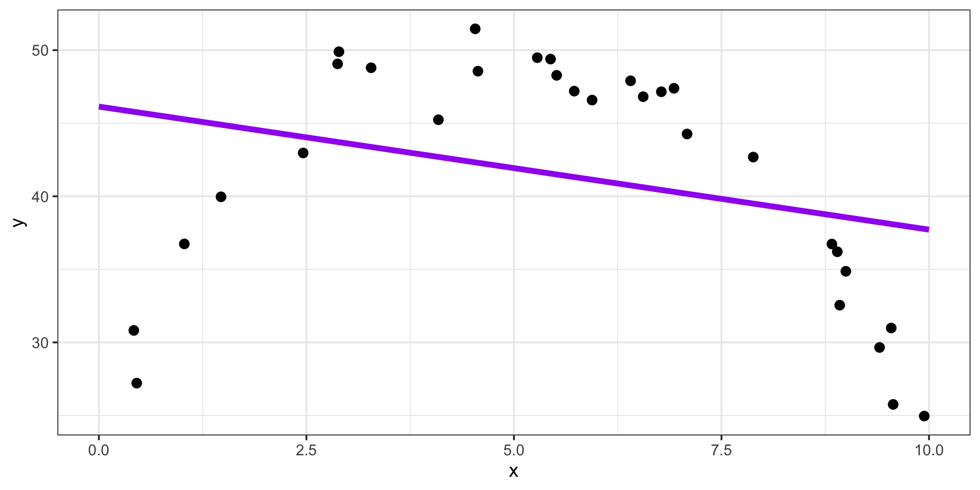
It is also possible for a model to have bias which is too high and variance which is too low

Consider the scenario below

The Connection Between Bias, Variance, and Model Flexibility

Models with high bias have low variance, and vice-versa.

• Decreasing bias by adding new \(\beta\)-parameters (allowing access to additional predictors, introducing dummy variables, polynomial terms, interactions, etc.) increases variance
• Bias and variance are in conflict with one another because they move in opposite directions

This is the bias/variance trade-off

Identifying an appropriate level of model flexibility means solving the bias/variance trade-off problem!

Overfitting and Underfitting

Let’s head back to the linear and eighth degree model from the opening slide again

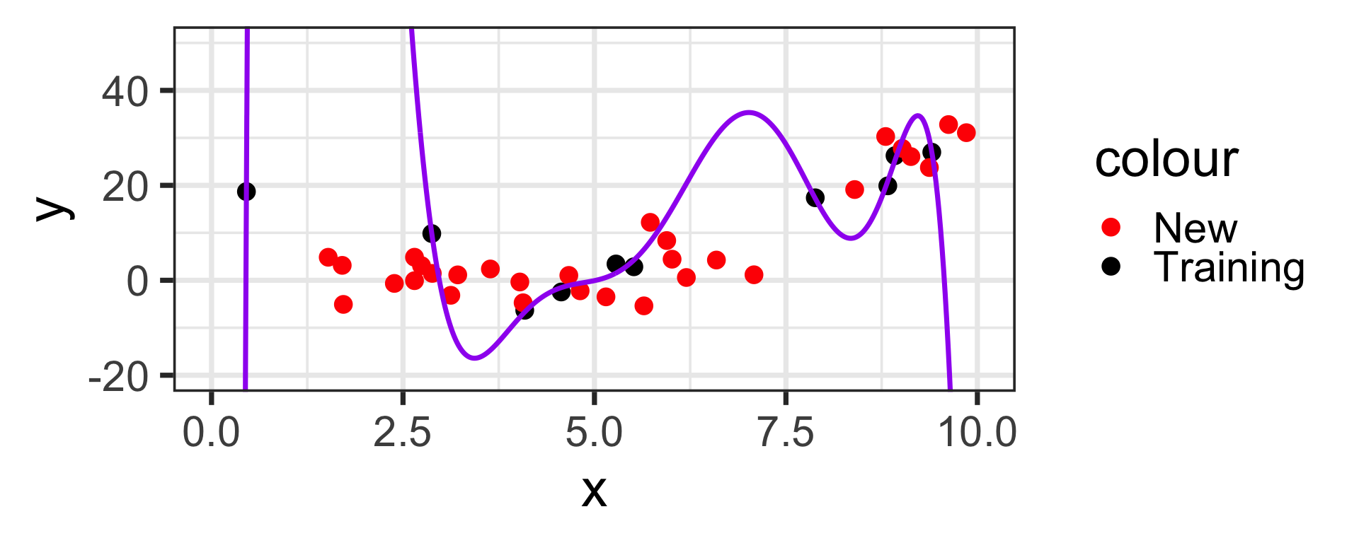
Now that we’ve fit these models, let’s see how they perform on new data drawn from the same population

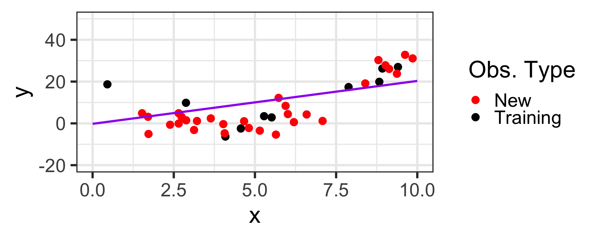
Underfit!

Overfit!

bias too high, variance too low

bias too low, variance to high

Not flexible enough

Too flexible

Training Error, Test Error, and Solving the Bias/Variance TradeOff Problem

Let’s start with a new data set, but I won’t tell you what degree association there is between \(x\) and \(y\)

Training Error, Test Error, and Solving the Bias/Variance TradeOff Problem

We’ll fit a variety of models

• Straight-line model
• Second-order (quadratic) model
• Third-order (cubic) model
• Fifth-order model
• Eleventh-order model

And then we’ll measure their performance

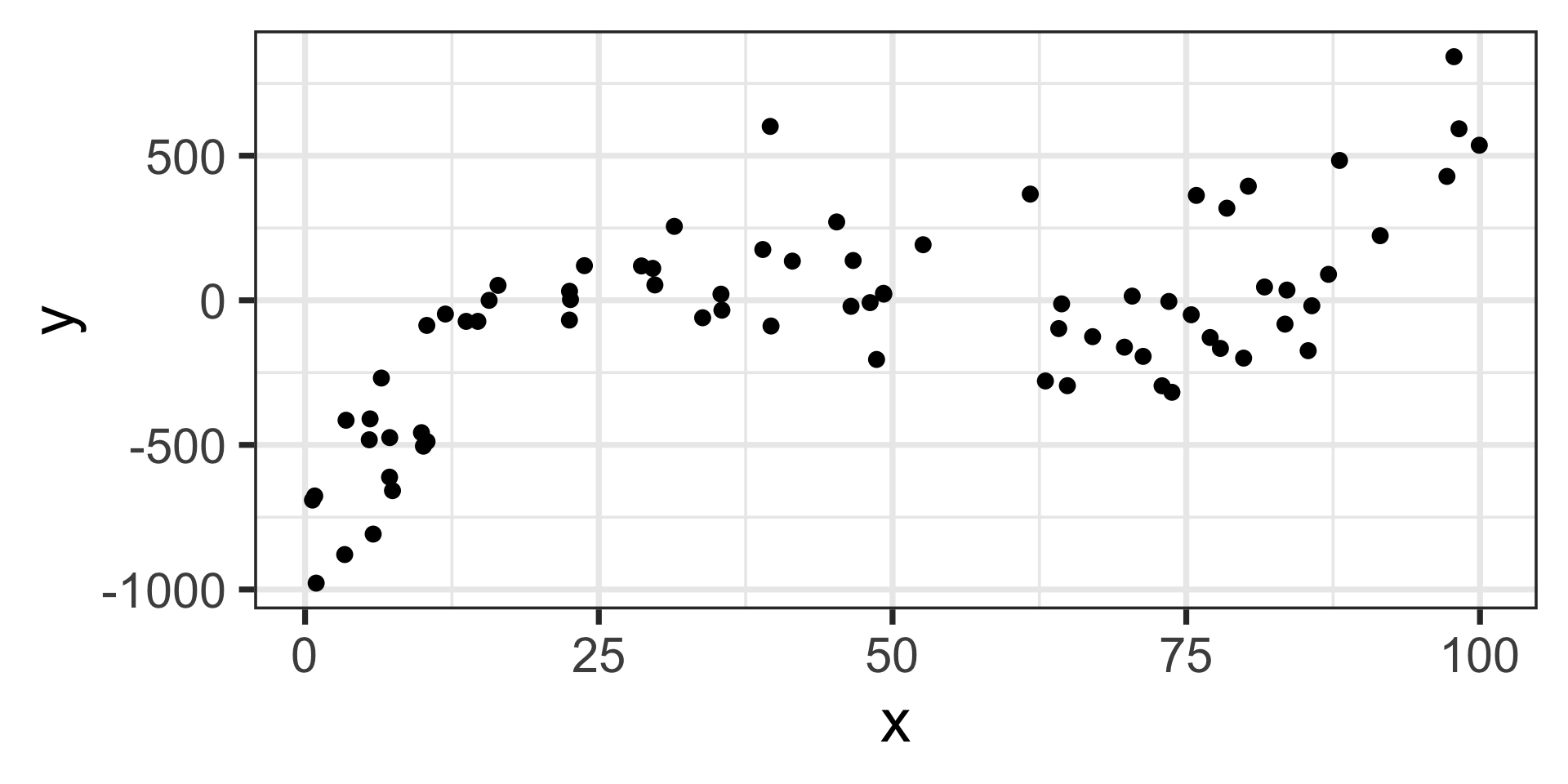
Training Error, Test Error, and Solving the Bias/Variance TradeOff Problem

Here they are…

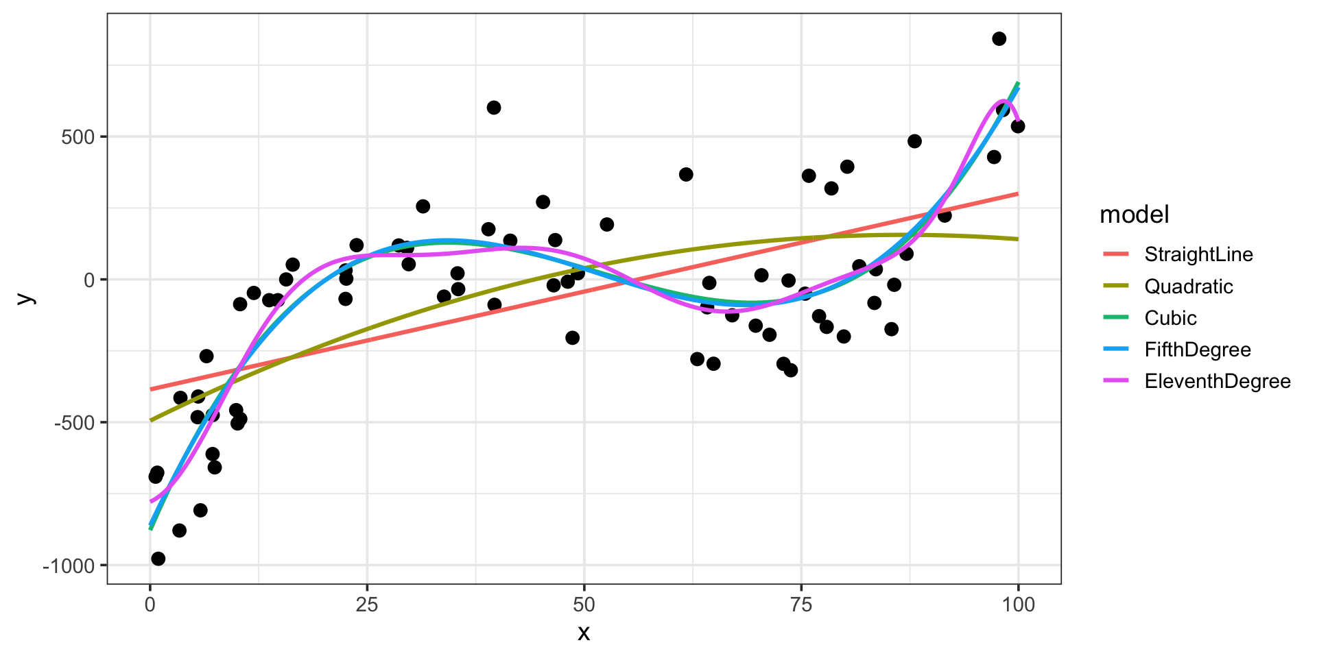
Training Error, Test Error, and Solving the Bias/Variance TradeOff Problem

Let’s examine the training metrics

model	degree	rsq	rmse
straight-line	1	0.1531330	272.4770
quadratic	2	0.1582909	271.6459
cubic	3	0.5636332	195.5906
5th-Order	5	0.5725649	193.5786
11th-order	11	0.5929268	188.9115

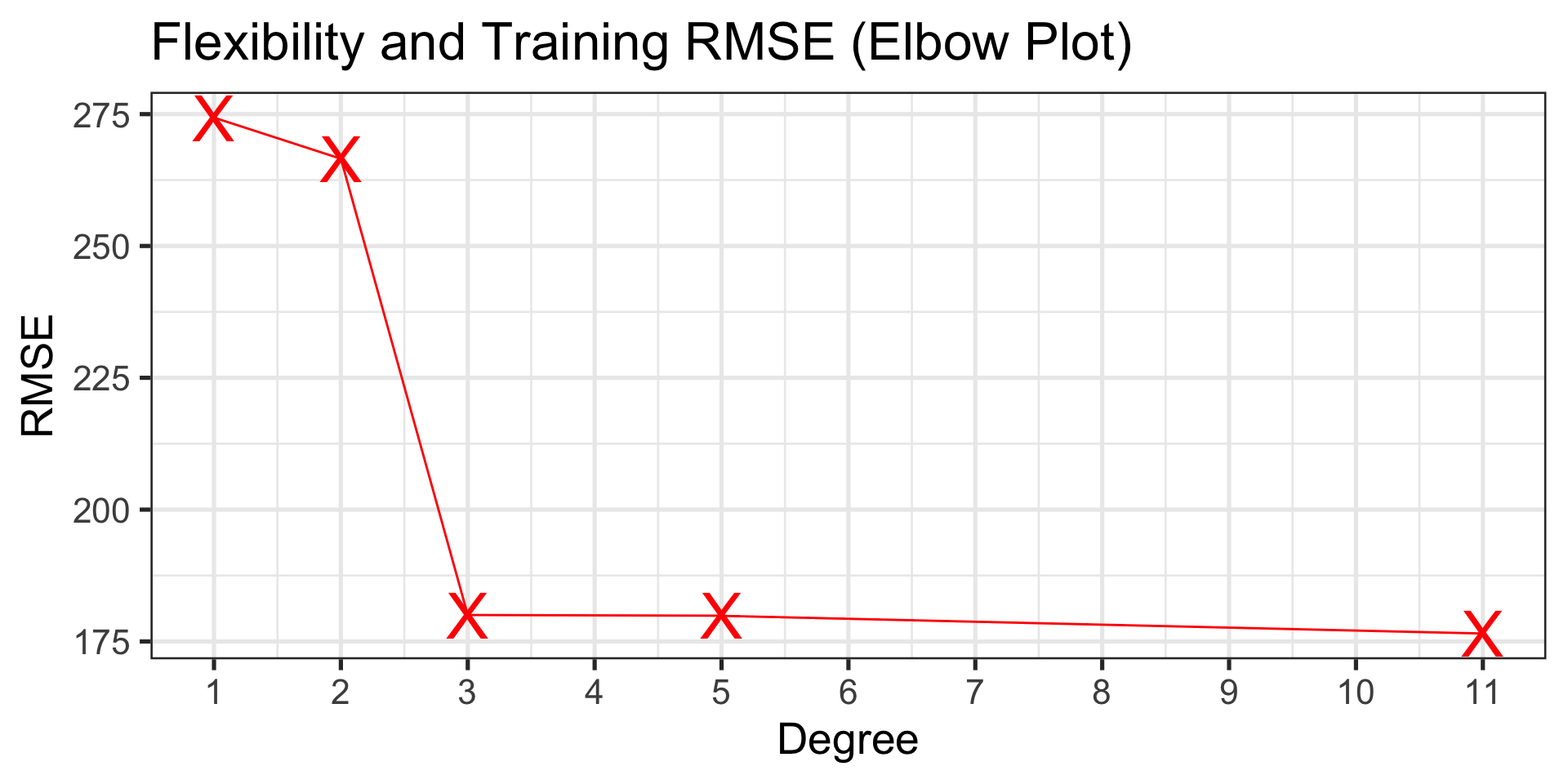
Performance gets better as flexibility increases!

Training Error, Test Error, and Solving the Bias/Variance TradeOff Problem

Let’s do the same with the test metrics

model	degree	rsq	rmse
straight-line	1	0.6029807	279.0266
quadratic	2	0.6210800	268.0826
cubic	3	0.7357107	194.5407
5th-Order	5	0.7176842	199.6257
11th-order	11	0.1710196	355.4256

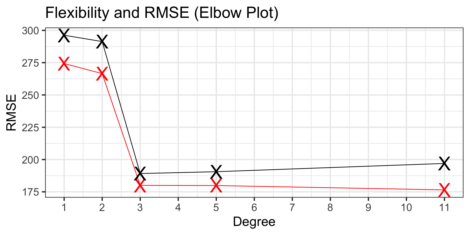
The training and test RMSE values largely agree over the lowest three levels of model flexibility, but…

Test performance gets worse with additional flexibility beyond third degree!

Training Error, Test Error, and Solving the Bias/Variance TradeOff Problem

Here’s the code I used to generate our toy dataset…

num_train <- 75
num_test <- 25
total_obs <- num_train + num_test

mystery_data <- tibble(
  x = runif(total_obs, 0, 100),
  y = 0.01*(x - 20)*(x - 60)*(x - 80) + rnorm(total_obs, 0, 200),
  type = c(rep("train", num_train), rep("test", num_test))
)

That’s a third-degree association!

Solving the Bias/Variance TradeOff Problem:

We can identify the appropriate level of model flexibility by finding the location of the bend in the elbow plot of test performance

Summary

• Bias and Variance are two competing measures on models

  • Models with high bias have low variance and are rigid/straight/flat – they are biased against complex associations
  • Models with low bias have high variance and are more “wiggly”

• Model variance refers to how much our model may change if provided a different training set from the same population

• Models with high variance are more flexible and are more likely to overfit

• Models with low variance are less flexible and are more likely to underfit

  • A model is overfit if it has learned too much about its training data and the model performance doesn’t generalize to unseen or new data

    • A telltale sign is if training performance is much better than test performance

  • A model is underfit if it is not flexible enough to capture the general trend between predictors and response

    • When training performance and test performance agree (or test performance is better than training performance), the model may be underfit

• We solve the bias/variance trade-off problem by finding the level of flexibility at which test performance is best (the bend in the elbow plot)

A Note About Optimal Flexibility

Remember that greater levels of flexibility are associated with

• a higher likelihood of overfitting
• greater difficulty in interpretation

If the improvements in model performance are small enough that they don’t outweigh these risks, we should choose the simpler (more parsimonious) model even if it doesn’t have the absolute best performance on the unseen test data

Next Time…

Cross-Validation