Interpretation of Marginal Effects with {marginaleffects}
October 25, 2024
Motivation
Recently, we’ve introduced utilization of higher-order terms to add flexibility to our models
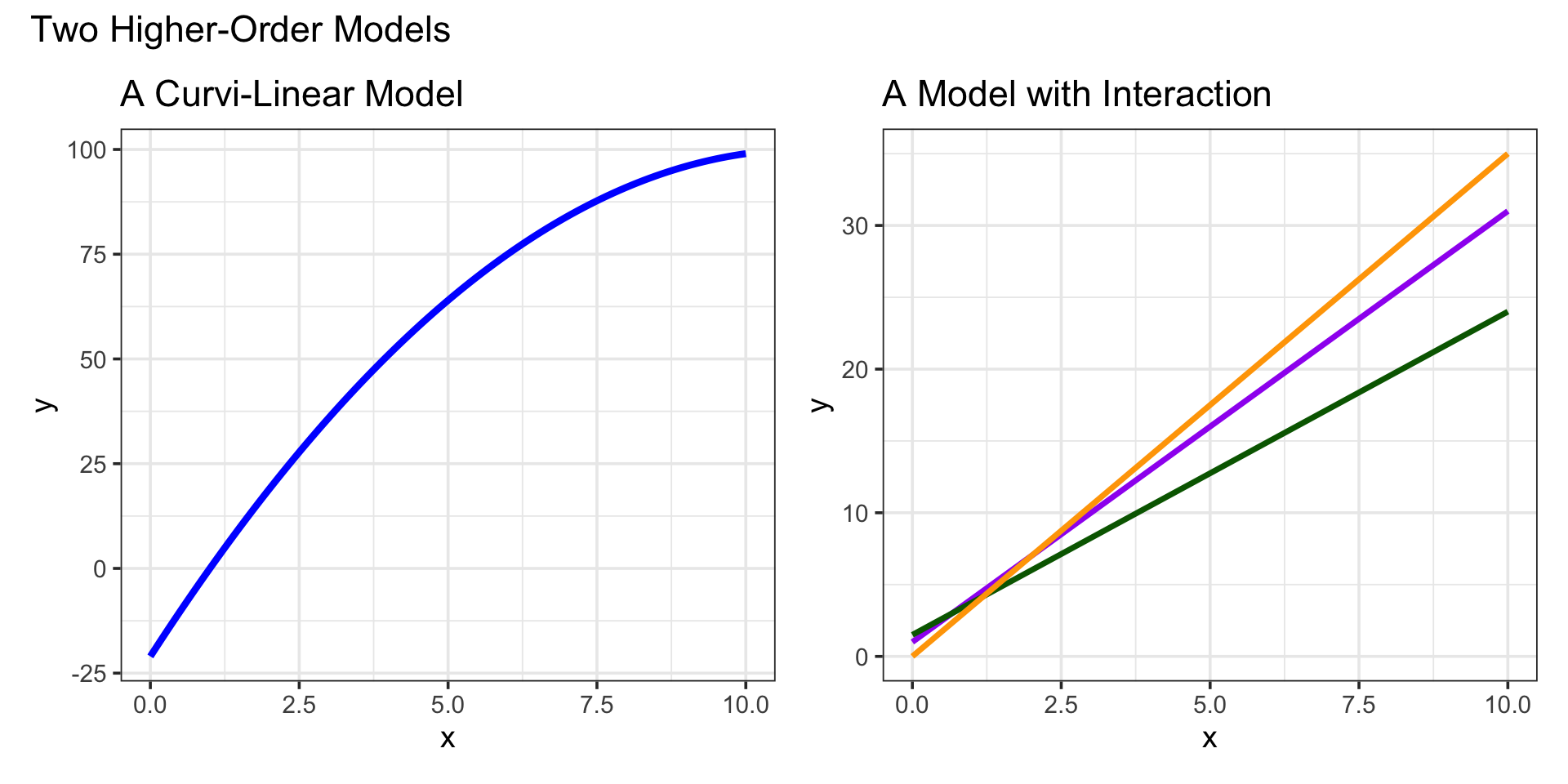
The use of these higher-order terms allows us to model more complex relationships between predictor(s) and our response, but this comes at costs…
Models including higher-order terms are more difficult to interpret
Note: There are other costs/risks too, but we’ll save those for another day
Marginal Effects for Simple Linear Regression
\[\mathbb{E}\left[y\right] = \beta_0 + \beta_1 \cdot x\]
We know what to expect here – the effect of a unit increase in \(x\) should be an expected increase in \(y\) by about \(\beta_1\)
That is, the marginal effect of \(x\) on \(y\) is constant, for this model
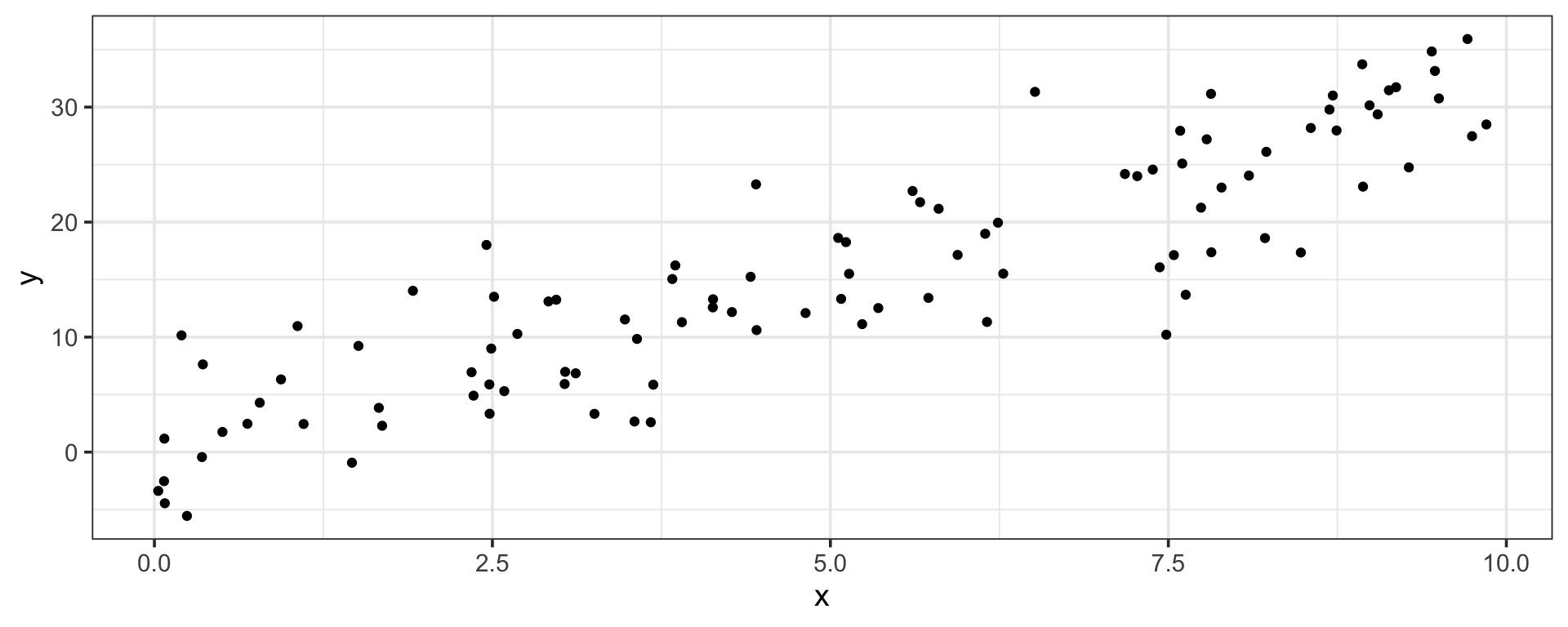
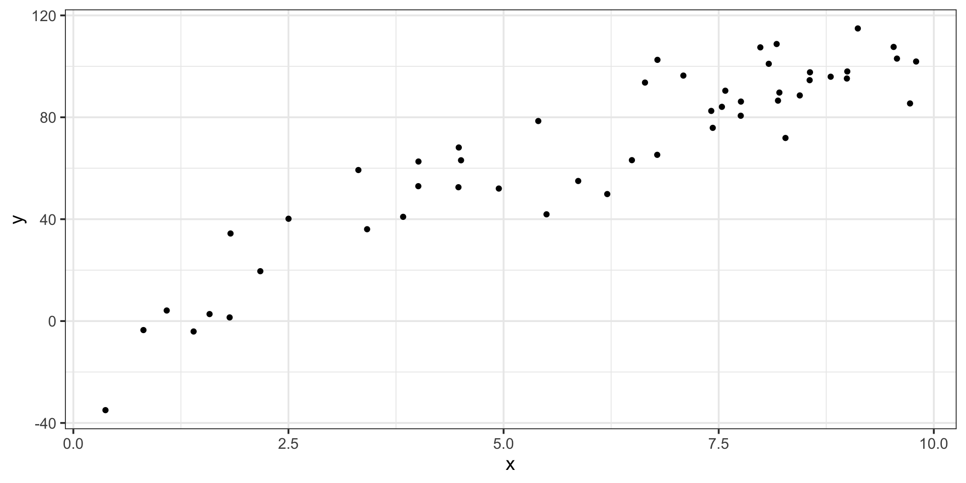
Let’s fit our simple linear regression model to this data and then examine the marginal effects
Marginal Effects for Simple Linear Regression
Code
| term | estimate | std.error | statistic | p.value |
|---|---|---|---|---|
| (Intercept) | 0.0789667 | 0.9303051 | 0.0848826 | 0.9325279 |
| x | 3.0606531 | 0.1593729 | 19.2043484 | 0.0000000 |
\[\mathbb{E}\left[y\right] = 0.079 + 3.06\cdot x\]
The estimated model appears below, on top of the training data.
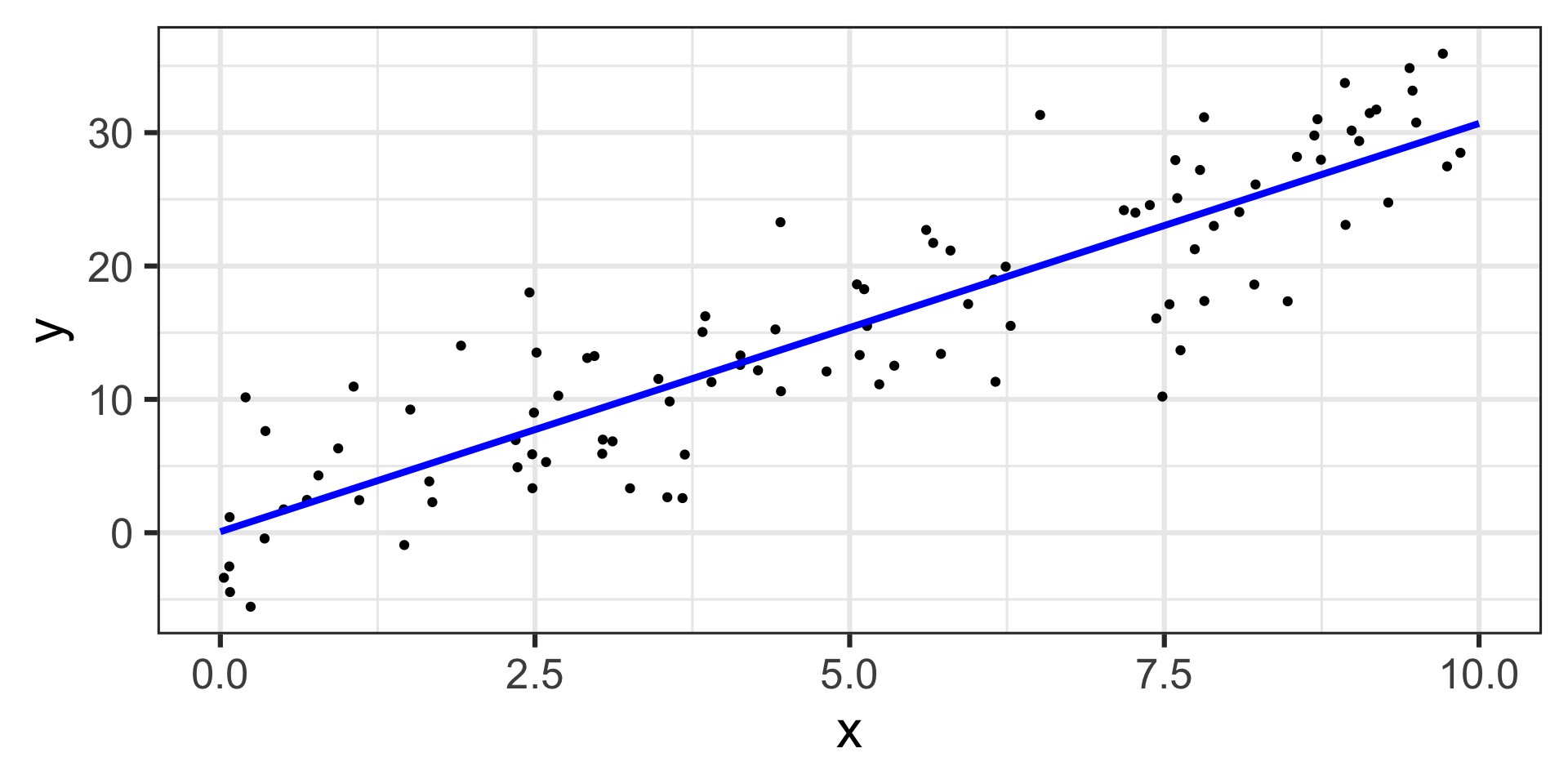
Now that we have our model, let’s use {marginaleffects} to determine the marginal effect of \(x\) on \(y\)
Code
mfx <- lr_fit %>%
  extract_fit_engine() %>%
  slopes(my_data) %>%
  tibble()

mfx %>%
  ggplot() +
  geom_ribbon(aes(x = x,
                  ymin = conf.low,
                  ymax = conf.high),
              fill = "grey",
              alpha = 0.5) +
  geom_line(aes(x = x,
                y = estimate),
            color = "black",
            linetype = "dashed") +
  coord_cartesian(
    ylim = c(-0.5, 5)
    ) +
  labs(x = "x",
       y = "Marginal Effect of x on y") +
  theme_bw(base_size = 24)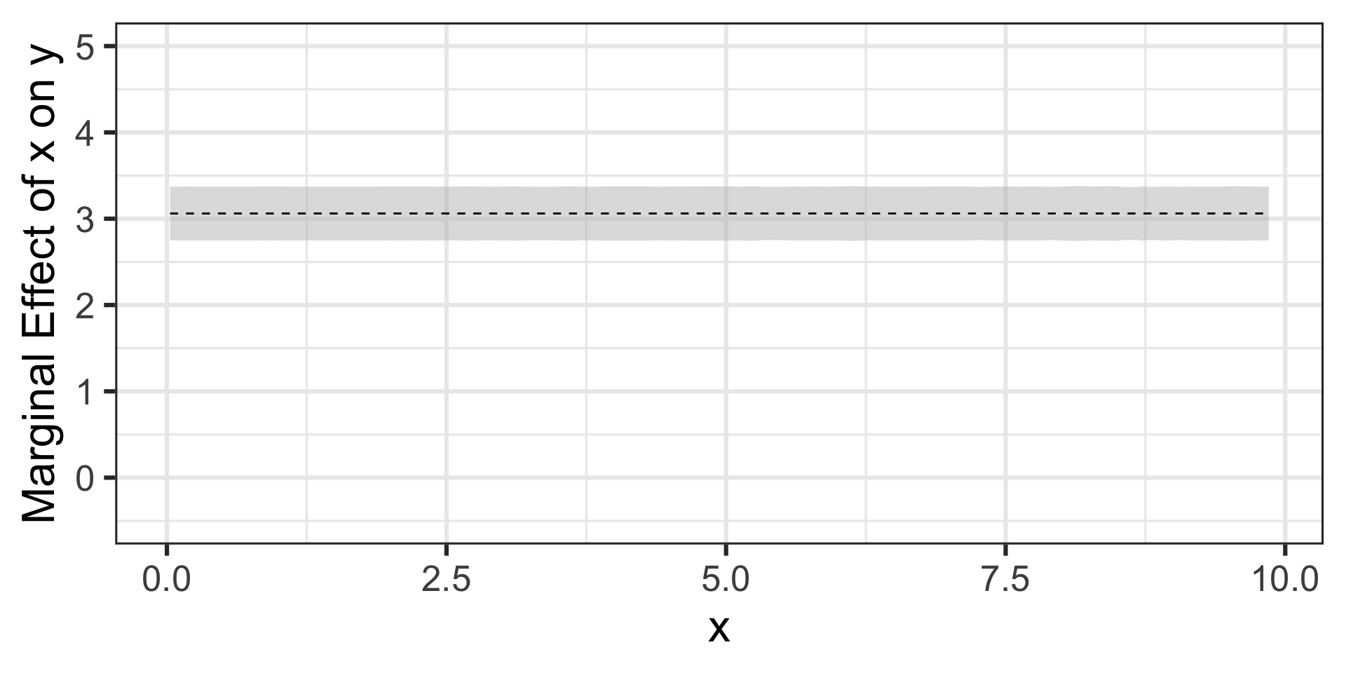
Marginal Effects for Simple Linear Regression
Code
| term | estimate | std.error | statistic | p.value |
|---|---|---|---|---|
| (Intercept) | 0.0789667 | 0.9303051 | 0.0848826 | 0.9325279 |
| x | 3.0606531 | 0.1593729 | 19.2043484 | 0.0000000 |
\[\mathbb{E}\left[y\right] = 0.079 + 3.06\cdot x\]
The estimated model appears below, on top of the training data.

As expected, a constant marginal effect at a height of \(\beta_1\)
Now that we have our model, let’s use {marginaleffects} to determine the marginal effect of \(x\) on \(y\)
Code
mfx <- lr_fit %>%
  extract_fit_engine() %>%
  slopes(my_data) %>%
  tibble()

mfx %>%
  ggplot() +
  geom_ribbon(aes(x = x,
                  ymin = conf.low,
                  ymax = conf.high),
              fill = "grey",
              alpha = 0.5) +
  geom_line(aes(x = x,
                y = estimate),
            color = "black",
            linetype = "dashed") +
  coord_cartesian(
    ylim = c(-0.5, 5)
    ) +
  labs(x = "x",
       y = "Marginal Effect of x on y") +
  theme_bw(base_size = 24)
Marginal Effects for a Model with a Quadratic Term
\[\mathbb{E}\left[y\right] = \beta_0 + \beta_1 x + \beta_2 x^2\]
Again, we know what to expect – the effect of a unit increase in \(x\) should be an expected increase in \(y\) by about \(\beta_1 + 2x\beta_2\)
That is, the marginal effect of \(x\) on \(y\) will change based on the value of \(x\) for this model
As we did with the last scenario, we’ll fit our model and examine the marginal effects
Marginal Effects for a Model with a Quadratic Term
Code
clr_spec <- linear_reg() %>%
  set_engine("lm")
clr_rec <- recipe(y ~ x, data = my_data) %>%
  step_poly(x, degree = 2, options = list(raw = TRUE))
clr_wf <- workflow() %>%
  add_model(clr_spec) %>%
  add_recipe(clr_rec)

clr_fit <- clr_wf %>%
  fit(my_data)

clr_fit %>%
  extract_fit_engine() %>%
  tidy() %>%
  kable() %>%
kable_styling(font_size = 16)| term | estimate | std.error | statistic | p.value |
|---|---|---|---|---|
| (Intercept) | -23.7867692 | 7.0140682 | -3.391294 | 0.0014188 |
| x_poly_1 | 21.8554094 | 2.9863758 | 7.318372 | 0.0000000 |
| x_poly_2 | -0.9402959 | 0.2744471 | -3.426146 | 0.0012810 |
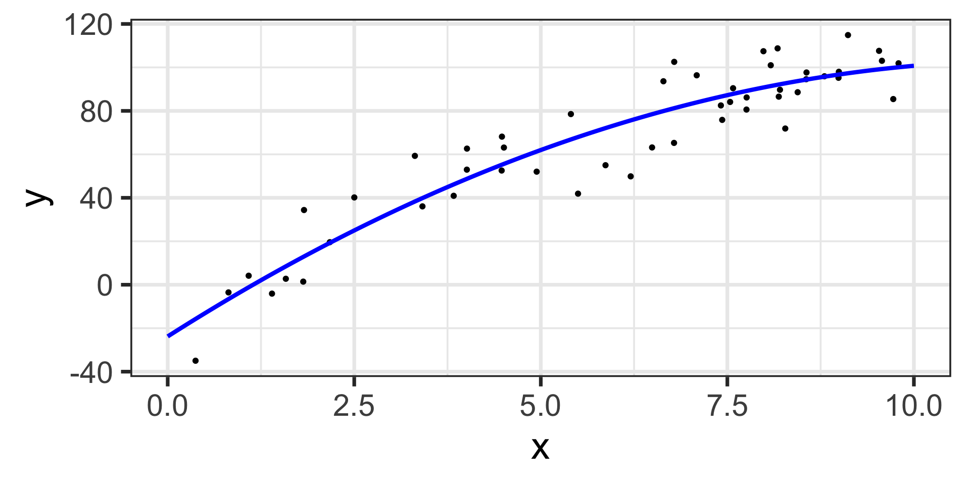
\[\mathbb{E}\left[y\right] = -23.79 + 21.86\cdot x - 0.94\cdot x^2\]
The estimated model appears below, on top of the training data.
Marginal Effects for a Model with a Quadratic Term
Code
clr_spec <- linear_reg() %>%
  set_engine("lm")
clr_rec <- recipe(y ~ x, data = my_data) %>%
  step_poly(x, degree = 2, options = list(raw = TRUE))
clr_wf <- workflow() %>%
  add_model(clr_spec) %>%
  add_recipe(clr_rec)

clr_fit <- clr_wf %>%
  fit(my_data)

clr_fit %>%
  extract_fit_engine() %>%
  tidy() %>%
  kable() %>%
kable_styling(font_size = 16)| term | estimate | std.error | statistic | p.value |
|---|---|---|---|---|
| (Intercept) | -23.7867692 | 7.0140682 | -3.391294 | 0.0014188 |
| x_poly_1 | 21.8554094 | 2.9863758 | 7.318372 | 0.0000000 |
| x_poly_2 | -0.9402959 | 0.2744471 | -3.426146 | 0.0012810 |
\[\mathbb{E}\left[y\right] = -23.79 + 21.86\cdot x - 0.94\cdot x^2\]
The estimated model appears below, on top of the training data.

Now that we have our model, let’s use {marginaleffects} to determine the marginal effect of \(x\) on \(y\)
Code
mfx <- slopes(clr_fit,
newdata = my_data,
variable = "x") %>%
tibble() %>%
mutate(x = my_data$x)
mfx %>%
ggplot() +
geom_ribbon(aes(x = x,
ymin = conf.low,
ymax = conf.high),
fill = "grey",
alpha = 0.5) +
geom_line(aes(x = x,
y = estimate),
color = "black",
linetype = "dashed") +
labs(x = "x",
y = "Marginal Effect of x on y") +
theme_bw(base_size = 24)
Marginal Effects for a Model with a Quadratic Term
Code
clr_spec <- linear_reg() %>%
  set_engine("lm")
clr_rec <- recipe(y ~ x, data = my_data) %>%
  step_poly(x, degree = 2, options = list(raw = TRUE))
clr_wf <- workflow() %>%
  add_model(clr_spec) %>%
  add_recipe(clr_rec)

clr_fit <- clr_wf %>%
  fit(my_data)

clr_fit %>%
  extract_fit_engine() %>%
  tidy() %>%
  kable() %>%
kable_styling(font_size = 16)| term | estimate | std.error | statistic | p.value |
|---|---|---|---|---|
| (Intercept) | -23.7867692 | 7.0140682 | -3.391294 | 0.0014188 |
| x_poly_1 | 21.8554094 | 2.9863758 | 7.318372 | 0.0000000 |
| x_poly_2 | -0.9402959 | 0.2744471 | -3.426146 | 0.0012810 |
\[\mathbb{E}\left[y\right] = -23.79 + 21.86\cdot x - 0.94\cdot x^2\]
The estimated model appears below, on top of the training data.

The marginal effect of \(x\) on \(y\) varies with the value of \(x\) – we can compute it using the expression \(\beta_1 + 2x\beta_2\)
Now that we have our model, let’s use {marginaleffects} to determine the marginal effect of \(x\) on \(y\)
Code
mfx <- slopes(clr_fit,
              newdata = my_data,
              variable = "x") %>%
  tibble() %>%
  mutate(x = my_data$x)

mfx %>%
  ggplot() +
  geom_ribbon(aes(x = x,
                  ymin = conf.low,
                  ymax = conf.high),
              fill = "grey",
              alpha = 0.5) +
  geom_line(aes(x = x,
                y = estimate),
            color = "black",
            linetype = "dashed") +
  labs(x = "x",
       y = "Marginal Effect of x on y") +
  theme_bw(base_size = 24)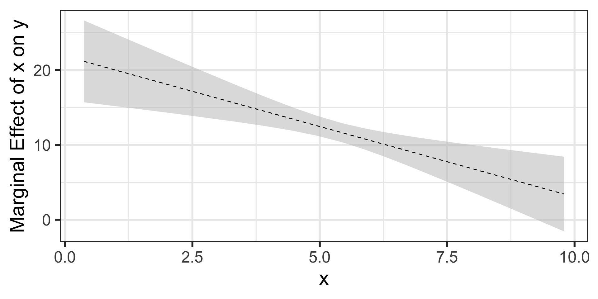
Marginal Effects for a Model with a Fifth-Degree Term
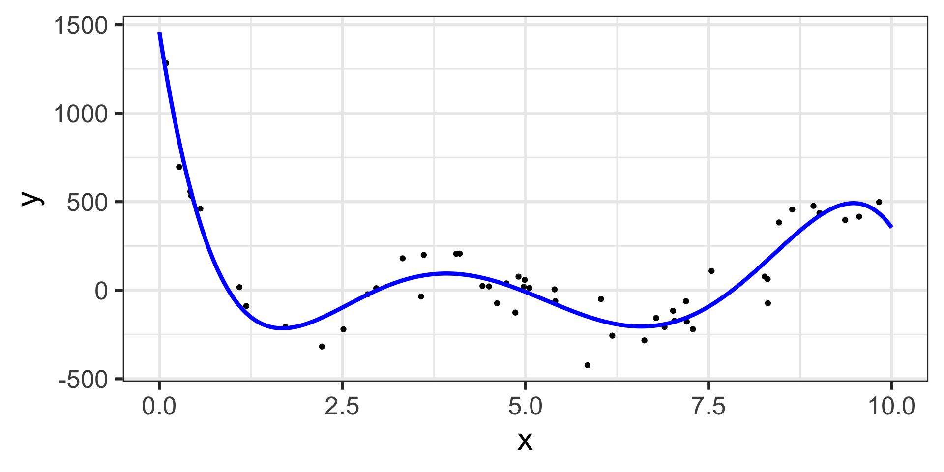
\[\mathbb{E}\left[y\right] = \beta_0 + \beta_1 x + \beta_2 x^2 + \beta_3 x^3 + \beta_4 x^4 + \beta_5 x^5\]
The effect of a unit increase in \(x\) here will be an expected increase in \(y\) of about \(\beta_1 + 2x\beta_2 + 3x^2\beta_3 + 4x^3\beta_4 + 5x^4\beta_5\)
Let’s see what {marginaleffects} does for us now…
Marginal Effects for a Model with a Fifth-Degree Term
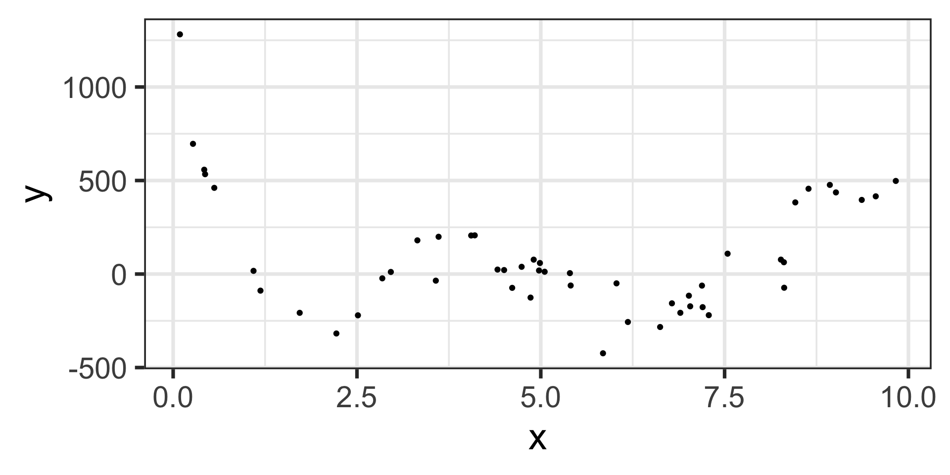
\[\mathbb{E}\left[y\right] = 1456.43 - 2656.07\cdot x + 1471.67\cdot x^2 - 342.64\cdot x^3 + 35.03\cdot x^4 - 1.29\cdot x^5\]
The estimated model appears below, on top of the training data.
Marginal Effects for a Model with a Fifth-Degree Term
\[\mathbb{E}\left[y\right] = 1456.43 - 2656.07\cdot x + 1471.67\cdot x^2 - 342.64\cdot x^3 + 35.03\cdot x^4 - 1.29\cdot x^5\]
The estimated model appears below, on top of the training data.

Now we’ll call on {marginaleffects}
Marginal Effects for a Model with a Fifth-Degree Term
\[\mathbb{E}\left[y\right] = 1456.43 - 2656.07\cdot x + 1471.67\cdot x^2 - 342.64\cdot x^3 + 35.03\cdot x^4 - 1.29\cdot x^5\]
The estimated model appears below, on top of the training data.

Now we’ll call on {marginaleffects}
Code
mfx <- slopes(c5lr_fit,
              newdata = my_data,
              variable = "x") %>%
  tibble() %>%
  mutate(x = my_data$x)

mfx %>%
  ggplot() +
  geom_ribbon(aes(x = x,
                  ymin = conf.low,
                  ymax = conf.high),
              fill = "grey",
              alpha = 0.5) +
  geom_line(aes(x = x,
                y = estimate),
            color = "black",
            linetype = "dashed") +
  labs(x = "x",
       y = "Marginal Effect of x on y") +
  theme_bw(base_size = 26)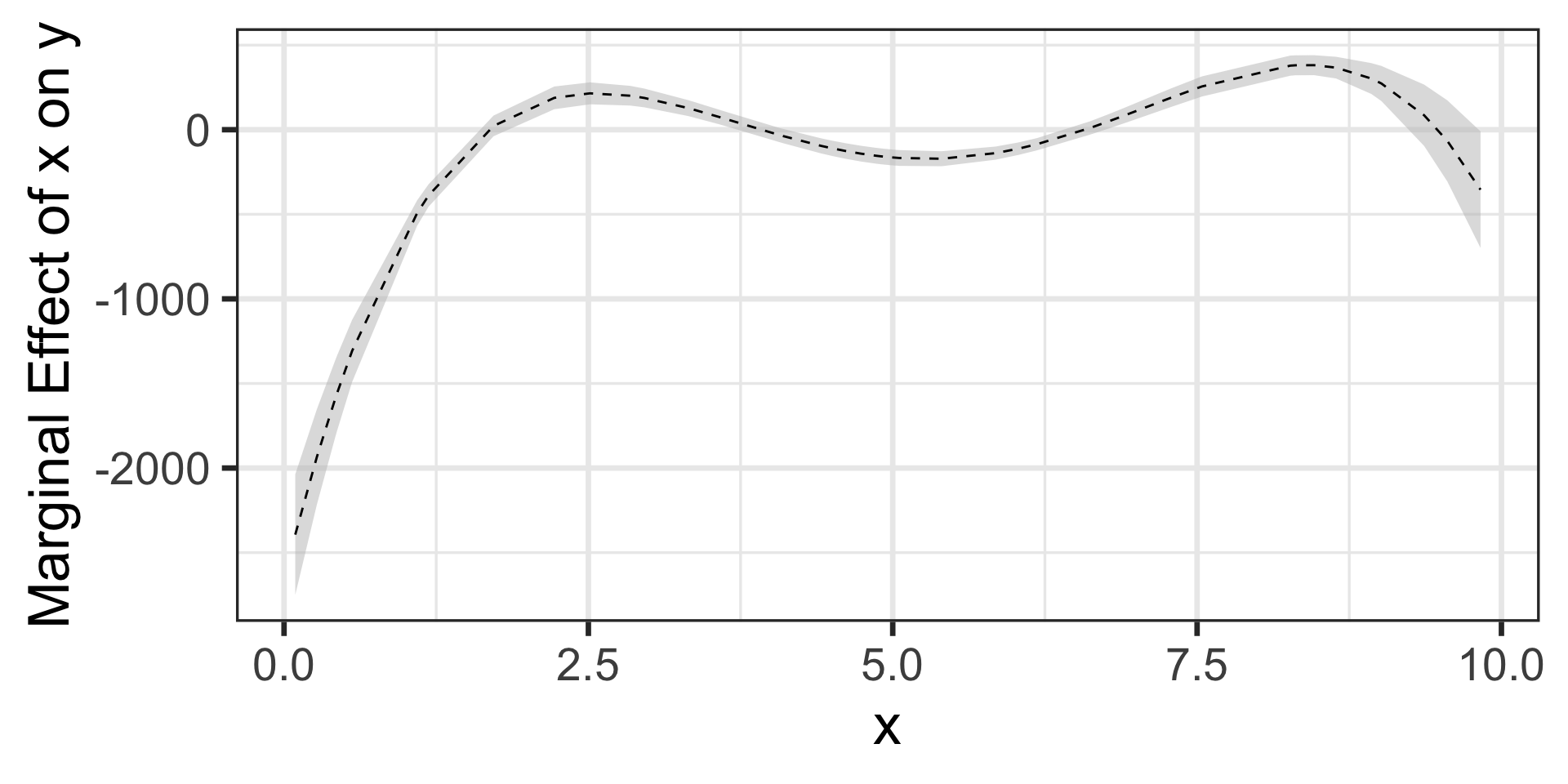
As in the case of the quadratic model we can see that the marginal effect of \(x\) on the response changes.
That is, the marginal effect of \(x\) on \(y\) depends on the “current” value of \(x\).
Marginal Effects for a Model with Linear Interactions
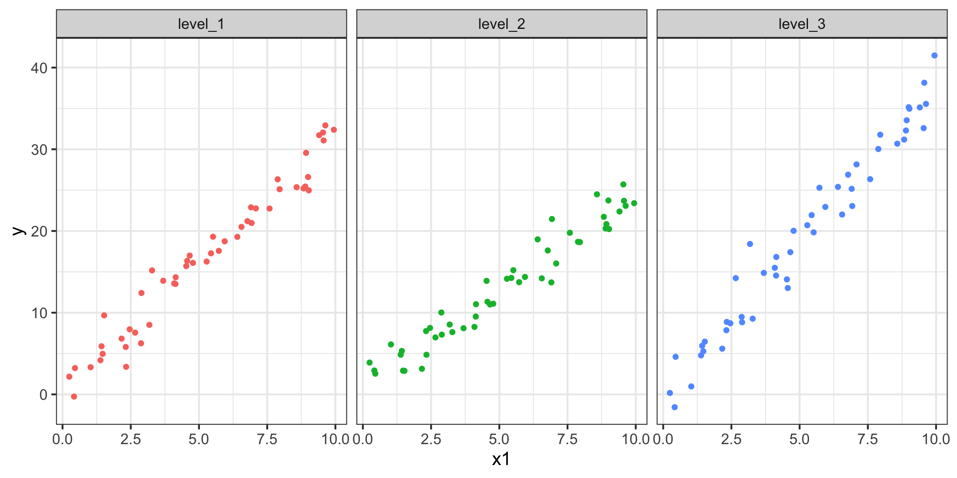
\[\mathbb{E}\left[y\right] = \beta_0 + \beta_1 x_1 + \beta_2\cdot\left(\text{level 2}\right) + \beta_3\cdot\left(\text{level 3}\right) + \beta_4\cdot x_1\left(\text{level 2}\right) + \beta_5\cdot x_1\left(\text{level 3}\right)\]
Here, we know that the effect of a unit increase in \(x_1\) depends on the observed level of \(x_2\)
That is, the marginal effect of \(x_1\) on \(y\) depends on the level of \(x_2\) – let’s see what {marginaleffects} gives us
Marginal Effects for a Model with Linear Interactions
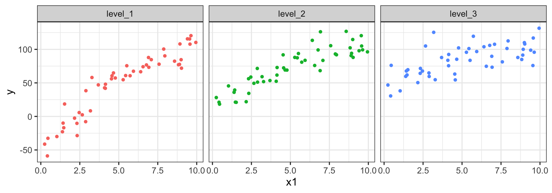
\[\mathbb{E}\left[y\right] = 0.72 + 3.08\cdot x_1 + 0.47\cdot \texttt{level2} - 1.04\cdot\texttt{level3} -0.76\cdot x_1\cdot\texttt{level2} + 0.73\cdot x_1\cdot\texttt{level3}\]
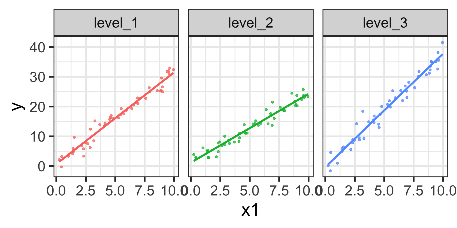
The estimated models are shown below.
Marginal Effects for a Model with Linear Interactions
\[\mathbb{E}\left[y\right] = 0.72 + 3.08\cdot x_1 + 0.47\cdot \texttt{level2} - 1.04\cdot\texttt{level3} -0.76\cdot x_1\cdot\texttt{level2} + 0.73\cdot x_1\cdot\texttt{level3}\]
The estimated models are shown below.

Let’s check on the marginal effects with {marginaleffects}
Code
mfx <- slopes(lr_fit,
              newdata = my_data,
              variable = "x1") %>%
  tibble() %>%
  mutate(x1 = my_data$x1,
         x2 = my_data$x2)

mfx %>%
  ggplot() +
  geom_ribbon(aes(x = x1,
                  ymin = conf.low,
                  ymax = conf.high),
              fill = "grey",
              alpha = 0.5) +
  geom_line(aes(x = x1,
                y = estimate),
            color = "black",
            linetype = "dashed") +
  labs(x = "x1",
       y = "Marginal Effect of x1 on y") +
  facet_wrap(~x2) +
  theme_bw(base_size = 28)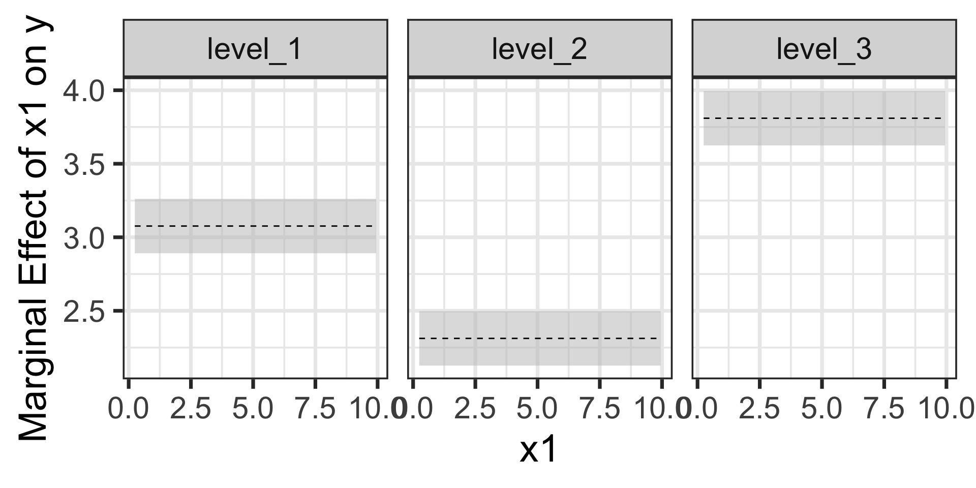
Marginal Effects for a Model with Linear Interactions
\[\mathbb{E}\left[y\right] = 0.72 + 3.08\cdot x_1 + 0.47\cdot \texttt{level2} - 1.04\cdot\texttt{level3} -0.76\cdot x_1\cdot\texttt{level2} + 0.73\cdot x_1\cdot\texttt{level3}\]
The estimated models are shown below.

We can see the differences in slopes (marginal effects) across the three levels of \(x_2\)
- level_1: \(\beta_1 \approx 3.08\)
- level_2: \(\beta_1 + \beta_4 \approx 3.08 - 0.76 = 2.32\)
- level_3: \(\beta_1 + \beta_5 \approx 3.08 + 0.73 = 3.81\)
Let’s check on the marginal effects with {marginaleffects}
Code
mfx <- slopes(lr_fit,
              newdata = my_data,
              variable = "x1") %>%
  tibble() %>%
  mutate(x1 = my_data$x1,
         x2 = my_data$x2)

mfx %>%
  ggplot() +
  geom_ribbon(aes(x = x1,
                  ymin = conf.low,
                  ymax = conf.high),
              fill = "grey",
              alpha = 0.5) +
  geom_line(aes(x = x1,
                y = estimate),
            color = "black",
            linetype = "dashed") +
  labs(x = "x1",
       y = "Marginal Effect of x1 on y") +
  facet_wrap(~x2) +
  theme_bw(base_size = 28)
Marginal Effects for a Model with Curvi-Linear Interactions
\[\begin{align} \mathbb{E}\left[y\right] = \beta_0 +~ &\beta_1 x_1 + \beta_2 x_1^2 + \beta_3\cdot\left(\text{level 2}\right) + \beta_4\cdot\left(\text{level 3}\right) +\\ &\beta_5\cdot x_1\left(\text{level 2}\right) + \beta_6\cdot x_1\left(\text{level 3}\right) +\\ &\beta_7\cdot x_1^2\left(\text{level 2}\right) + \beta_8\cdot x_1^2\left(\text{level 3}\right)\end{align}\]
Let’s fit the model and see how {marginaleffects} helps us analyze the expected effect of a unit change in \(x_1\) across the different levels of \(x_2\)
Marginal Effects for a Model with Curvi-Linear Interactions
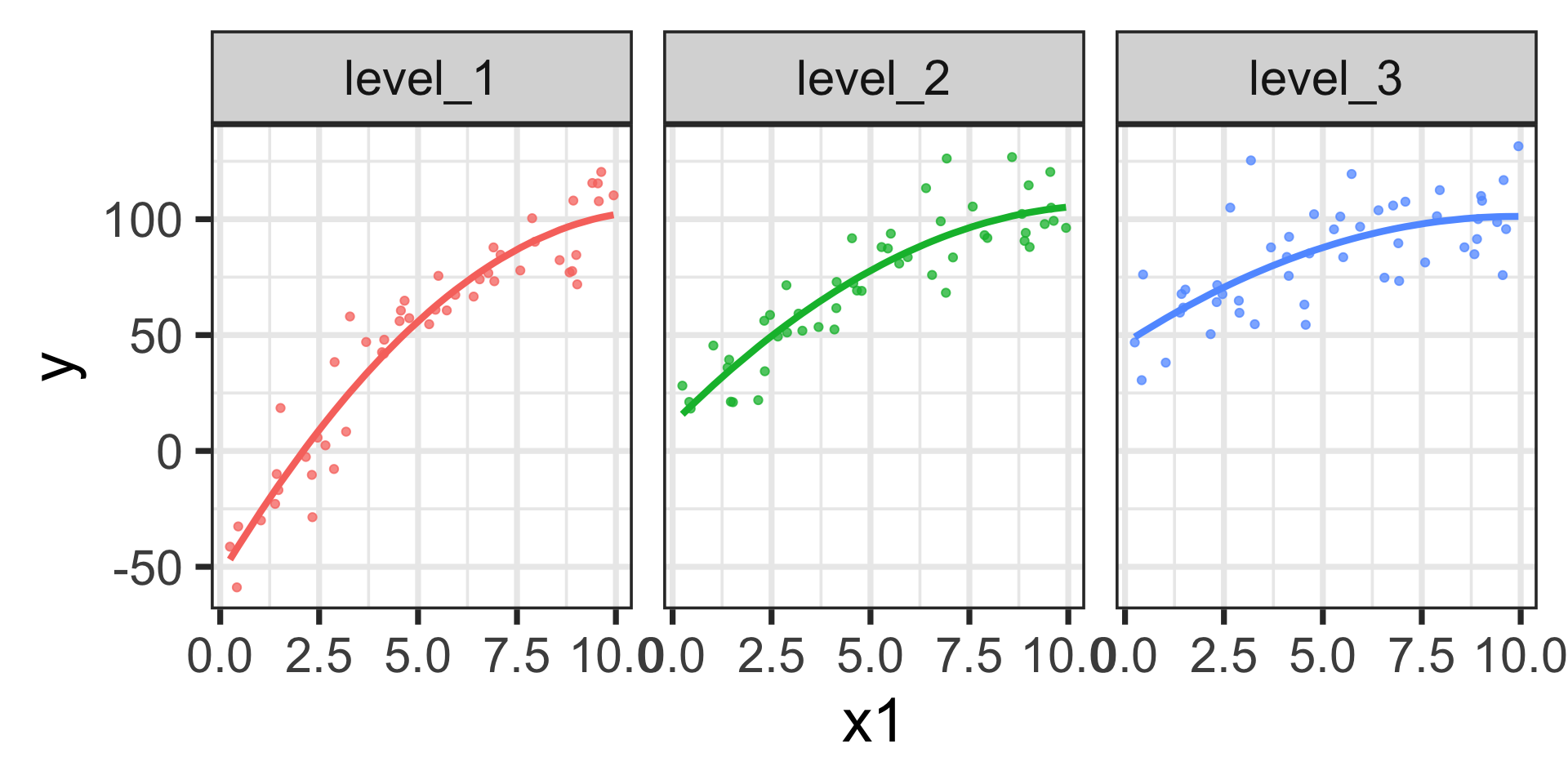
\[\begin{align} \mathbb{E}\left[y\right] = -53.77 +~ &28.28 x_1 - 1.27x_1^2 + 65.42\cdot\left(\text{level 2}\right) + 100.22\cdot\left(\text{level 3}\right) +\\ &-11.19\cdot x_1\left(\text{level 2}\right) - 17.22\cdot x_1\left(\text{level 3}\right) +\\ &0.50\cdot x_1^2\left(\text{level 2}\right) + 0.71\cdot x_1^2\left(\text{level 3}\right)\end{align}\]
Again, the estimated models are shown below.

Marginal Effects for a Model with Curvi-Linear Interactions
\[\begin{align} \mathbb{E}\left[y\right] = -53.77 +~ &28.28 x_1 - 1.27x_1^2 + 65.42\cdot\left(\text{level 2}\right) + 100.22\cdot\left(\text{level 3}\right) +\\ &-11.19\cdot x_1\left(\text{level 2}\right) - 17.22\cdot x_1\left(\text{level 3}\right) +\\ &0.50\cdot x_1^2\left(\text{level 2}\right) + 0.71\cdot x_1^2\left(\text{level 3}\right)\end{align}\]
Again, the estimated models are shown below.

Unsurprisingly, we’ll use {marginaleffects} to check in on the marginal effect of \(x_1\) on \(y\).
Marginal Effects for a Model with Curvi-Linear Interactions
\[\begin{align} \mathbb{E}\left[y\right] = -53.77 +~ &28.28 x_1 - 1.27x_1^2 + 65.42\cdot\left(\text{level 2}\right) + 100.22\cdot\left(\text{level 3}\right) +\\ &-11.19\cdot x_1\left(\text{level 2}\right) - 17.22\cdot x_1\left(\text{level 3}\right) +\\ &0.50\cdot x_1^2\left(\text{level 2}\right) + 0.71\cdot x_1^2\left(\text{level 3}\right)\end{align}\]
Again, the estimated models are shown below.
Unsurprisingly, we’ll use {marginaleffects} to check in on the marginal effect of \(x_1\) on \(y\).
Code
mfx <- slopes(lr_fit,
              newdata = my_data,
              variable = "x1") %>%
  tibble() %>%
  mutate(x1 = my_data$x1,
         x2 = my_data$x2)

mfx %>%
  ggplot() +
  geom_ribbon(aes(x = x1,
                  ymin = conf.low,
                  ymax = conf.high),
              fill = "grey",
              alpha = 0.5) +
  geom_line(aes(x = x1,
                y = estimate),
            color = "black",
            linetype = "dashed") +
  labs(x = "x1",
       y = "Marginal Effect of x1 on y") +
  facet_wrap(~x2) +
  theme_bw(base_size = 28)
Marginal Effects for a Model with Curvi-Linear Interactions
\[\begin{align} \mathbb{E}\left[y\right] = -53.77 +~ &28.28 x_1 - 1.27x_1^2 + 65.42\cdot\left(\text{level 2}\right) + 100.22\cdot\left(\text{level 3}\right) +\\ &-11.19\cdot x_1\left(\text{level 2}\right) - 17.22\cdot x_1\left(\text{level 3}\right) +\\ &0.50\cdot x_1^2\left(\text{level 2}\right) + 0.71\cdot x_1^2\left(\text{level 3}\right)\end{align}\]
Again, the estimated models are shown below.

We can see the differences in slopes (marginal effects) and the differences in change in slopes across the three levels of \(x_2\) here. We could still evaluate the marginal effects using calculus if we wanted to.
Unsurprisingly, we’ll use {marginaleffects} to check in on the marginal effect of \(x_1\) on \(y\).
Code
mfx <- slopes(lr_fit,
              newdata = my_data,
              variable = "x1") %>%
  tibble() %>%
  mutate(x1 = my_data$x1,
         x2 = my_data$x2)

mfx %>%
  ggplot() +
  geom_ribbon(aes(x = x1,
                  ymin = conf.low,
                  ymax = conf.high),
              fill = "grey",
              alpha = 0.5) +
  geom_line(aes(x = x1,
                y = estimate),
            color = "black",
            linetype = "dashed") +
  labs(x = "x1",
       y = "Marginal Effect of x1 on y") +
  facet_wrap(~x2) +
  theme_bw(base_size = 28)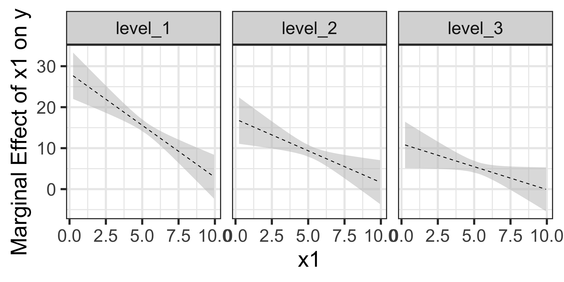
Marginal Effects for a Model with Curvi-Linear Interactions
\[\begin{align} \mathbb{E}\left[y\right] = -53.77 +~ &28.28 x_1 - 1.27x_1^2 + 65.42\cdot\left(\text{level 2}\right) + 100.22\cdot\left(\text{level 3}\right) +\\ &-11.19\cdot x_1\left(\text{level 2}\right) - 17.22\cdot x_1\left(\text{level 3}\right) +\\ &0.50\cdot x_1^2\left(\text{level 2}\right) + 0.71\cdot x_1^2\left(\text{level 3}\right)\end{align}\]
Again, the estimated models are shown below.

We can see the differences in slopes (marginal effects) and the differences in change in slopes across the three levels of \(x_2\) here. We could still evaluate the marginal effects using calculus if we wanted to.
Unsurprisingly, we’ll use {marginaleffects} to check in on the marginal effect of \(x_1\) on \(y\).
Code
mfx <- slopes(lr_fit,
              newdata = my_data,
              variable = "x1") %>%
  tibble() %>%
  mutate(x1 = my_data$x1,
         x2 = my_data$x2)

mfx %>%
  ggplot() +
  geom_ribbon(aes(x = x1,
                  ymin = conf.low,
                  ymax = conf.high),
              fill = "grey",
              alpha = 0.5) +
  geom_line(aes(x = x1,
                y = estimate),
            color = "black",
            linetype = "dashed") +
  labs(x = "x1",
       y = "Marginal Effect of x1 on y") +
  facet_wrap(~x2) +
  theme_bw(base_size = 28)
What was challenging to investigate without calculus is made easier with {marginaleffects}