Higher-Order Terms: Interactions in Regression
October 22, 2024
Motivation
Motivation
In our first discussion on higher-order terms, we saw how to use polynomial terms in regression models
- We use polynomial terms when the expected change in the response due to a change in the value of a predictor changes depending on the “current” value of the predictor
- That is, the expected change in the response due to a change in the predictor is not constant
There is another way for an association between predictor and response to be non-constant…
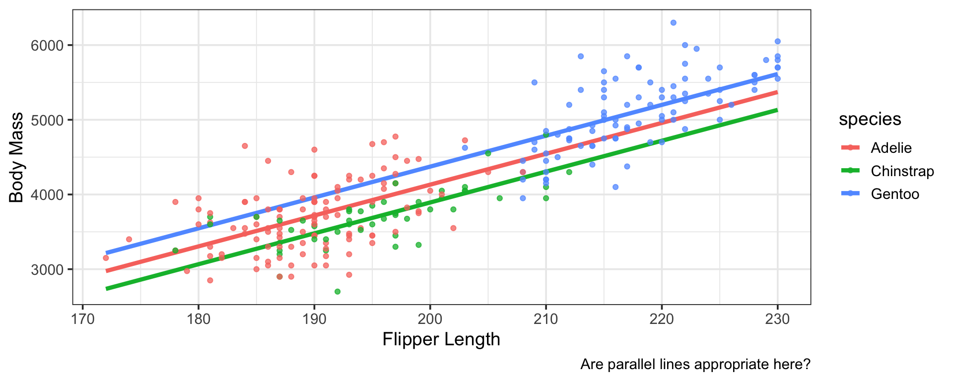
What if the effect of a change in one predictor on the response depends on the value of another predictor, as we came to suspect with flipper length, species, and body mass on the previous slide?
We can handle this scenario using interactions
Types of Interactions
There are three main types of two-way interactions
- Categorical-Categorical: An interaction between two categorical variables
- Categorical-Numerical: An interaction between a categorical variable and a numerical variable
- Numerical-Numerical: An interaction between two numerical variables
We’ll see what each one accommodates and how to implement each type of interaction here
A Note Before Moving Forward
This notebook omits both global assessments of model utility and individual term-based assessments in order to focus on the types of interactions available to us, why we use them, and what phenomena we are trying to model when we use a particular type of interaction
As with all previously discussed topics, we conduct term-based assessments and remove individual terms which are insignificant, one at a time, in order of highest \(p\)-value to lowest
If a higher order term (ie. an interaction) is deemed significant, then all of its component lower order terms must be kept in the model, regardless of statistical significance
Playing Along
Hopefully, you’ve become accustomed to playing along with the used cars data set (or another data set you find more interesting) during our discussions. I encourage you to continue doing this.
- Open RStudio and verify that you are working within your
MAT300project - Open the notebook you’ve been building onto since we began with our first discussion on simple linear regression
- Run all of the code in the notebook
- Add a section on models with interaction terms
Reminder: Models with Categorical Predictors
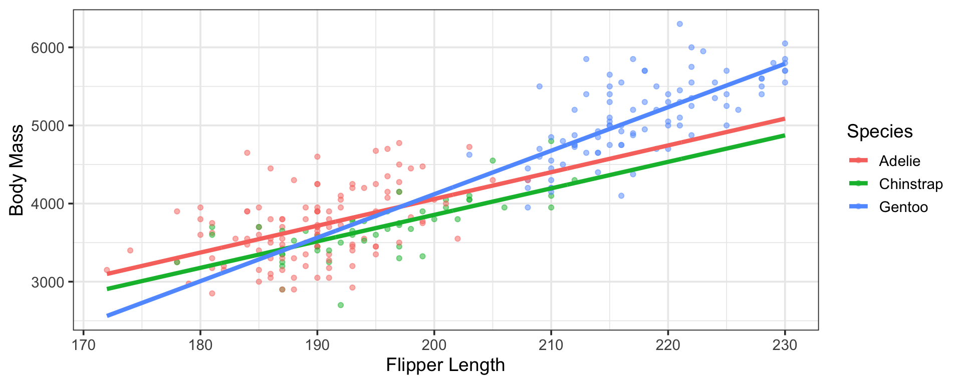
Recall that the effect of including a categorical predictor in a model is an adjustment in the model intercept for each category.
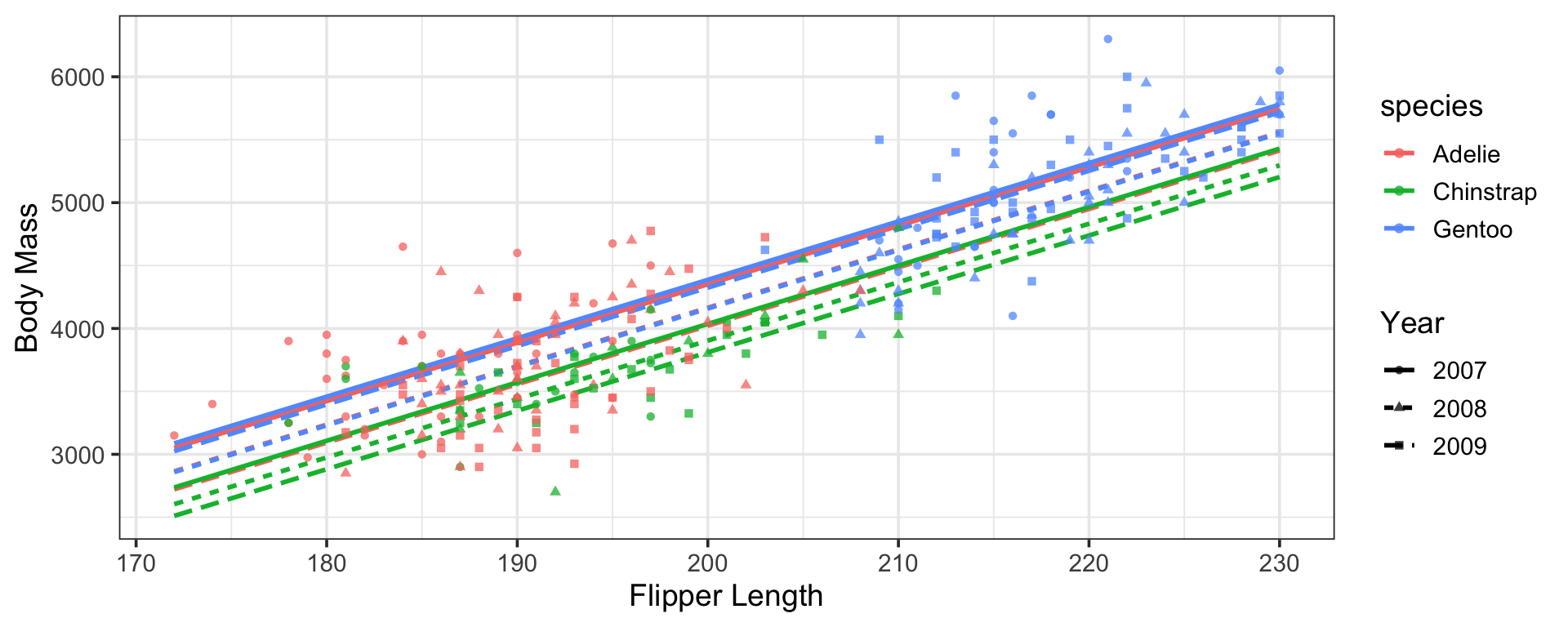
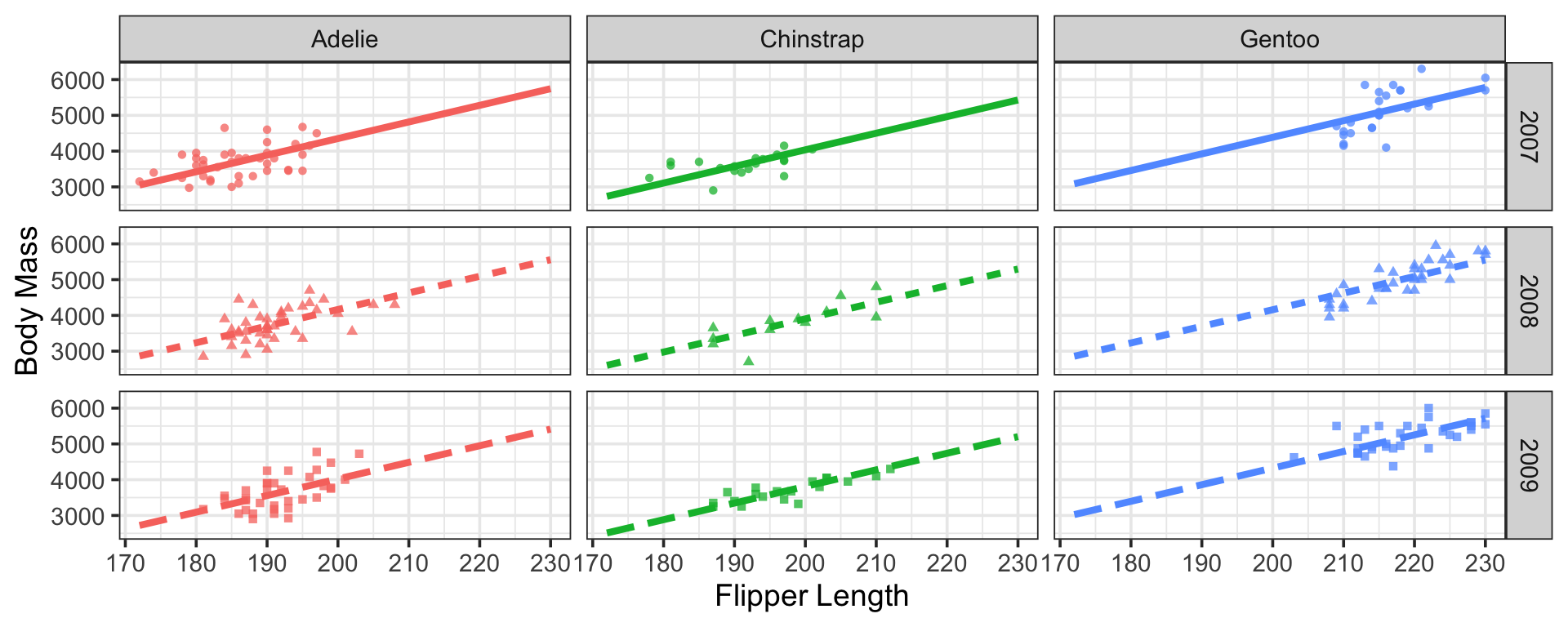
Below are visual representations of two models, both using flipper length as predictors but one using species as an additional predictor of body mass and the other using year
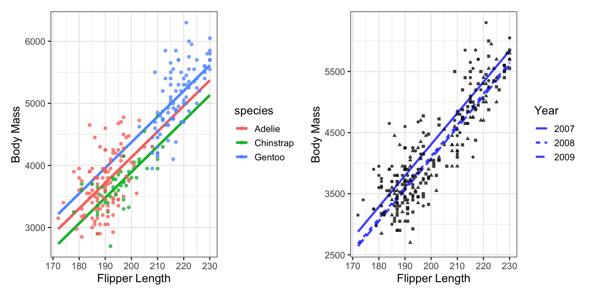
Models with Categorical Predictors (Cont’d.)
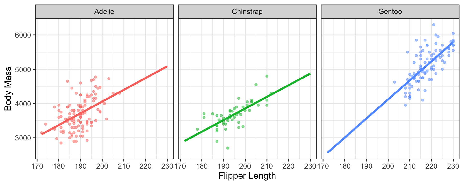
We could even build a model that compensates for both species and year simultaneously
A visual of such a model appears below
Models with Categorical Predictors (Cont’d.)
Let’s take a look at this new fitted model
| term | estimate | std.error | statistic | p.value |
|---|---|---|---|---|
| (Intercept) | -4905.72228 | 692.112621 | -7.088040 | 0.0000000 |
| flipper_length_mm | 46.09867 | 3.700356 | 12.457901 | 0.0000000 |
| year_X2008 | -195.30117 | 59.256639 | -3.295853 | 0.0011235 |
| year_X2009 | -209.68399 | 59.547650 | -3.521281 | 0.0005103 |
| species_Chinstrap | -270.54493 | 66.179394 | -4.088054 | 0.0000587 |
| species_Gentoo | 117.90795 | 115.092591 | 1.024462 | 0.3066075 |
\[\scriptsize{\begin{align} \mathbb{E}\left[\text{body mass}\right] \approx -4905.72 +~ &46.1\cdot\left(\text{flipper length}\right) - 195.3\cdot\left(\text{year2008}\right) +\\ &- 209.68\cdot\left(\text{year2009}\right) - 270.54\cdot\left(\text{speciesChinstrap}\right) +\\ & 117.91\cdot\left(\text{speciesGentoo}\right)\end{align}}\]
We can see, mathematically, that this model assumes an effect for species and an effect for year on penguin body mass, independently of one another
That is, year-to-year, all penguins body masses are impacted in the same way, regardless of species
Interactions Between Categorical Predictors
It would be reasonable to ask whether yearly conditions had different impacts across the species of penguin
We can answer this by constructing and analysing a model that includes an interaction between year and species
We can compare the previous model form to this proposed model form below.
Model with Year and Species Independently:
\[\scriptsize{\begin{align} \mathbb{E}\left[\text{body mass}\right] \approx \beta_0 +~ &\beta_1\cdot\left(\text{flipper length}\right) + \beta_2\cdot\left(\text{year2008}\right) + \beta_3\cdot\left(\text{year2009}\right) +\\ &\beta_4\cdot\left(\text{speciesChinstrap}\right) + \beta_5\cdot\left(\text{speciesGentoo}\right)\end{align}}\]
Model with Interaction Between Year and Species:
\[\scriptsize{\begin{align} \mathbb{E}\left[\text{body mass}\right] \approx \beta_0 +~ &\beta_1\cdot\left(\text{flipper length}\right) + \beta_2\cdot\left(\text{year2008}\right) + \beta_3\cdot\left(\text{year2009}\right) +\\ &\beta_4\cdot\left(\text{speciesChinstrap}\right) + \beta_5\cdot\left(\text{speciesGentoo}\right) +\\ &\beta_6\cdot\left(\text{speciesGentoo}\cdot\text{year2008}\right) +\\ &\beta_7\cdot\left(\text{speciesGentoo}\cdot\text{year2009}\right) +\\ &\beta_8\cdot\left(\text{speciesChinstrap}\cdot\text{year2008}\right) +\\ &\beta_9\cdot\left(\text{speciesChinstrap}\cdot\text{year2009}\right) \end{align}}\]
Building a Model with Interactions
In {tidymodels}, we use step_interact() as part of our recipe to create an interaction
mlr_flsy_isy_spec <- linear_reg() %>%
  set_engine("lm")

mlr_flsy_isy_rec <- recipe(body_mass_g ~ flipper_length_mm + species + year,
                           data = penguins_train) %>%
  step_mutate(year = as.factor(year)) %>%
  step_dummy(year) %>%
  step_dummy(species) %>%
  step_interact(~ starts_with("species"):starts_with("year"))

mlr_flsy_isy_wf <- workflow() %>%
  add_model(mlr_flsy_isy_spec) %>%
  add_recipe(mlr_flsy_isy_rec)

mlr_flsy_isy_fit <- mlr_flsy_isy_wf %>%
  fit(penguins_train)
Building a Model with Interactions
\(\bigstar\) Let’s try it! \(\bigstar\)
- Choose two categorical variables and one numerical variable to use in predicting the rental price of an Air BnB
- Build the corresponding model specification and recipe which will accommodate an interaction between the two categorical predictors
- Package your specification and recipe together into a workflow
- Fit your workflow to your training data
The Estimated Model
| term | estimate | std.error | statistic | p.value |
|---|---|---|---|---|
| (Intercept) | -4933.59608 | 691.592270 | -7.1336773 | 0.0000000 |
| flipper_length_mm | 46.42457 | 3.704239 | 12.5328209 | 0.0000000 |
| year_X2008 | -186.53149 | 84.902008 | -2.1970209 | 0.0289520 |
| year_X2009 | -330.22761 | 88.313278 | -3.7392747 | 0.0002296 |
| species_Chinstrap | -315.26370 | 104.431973 | -3.0188427 | 0.0028044 |
| species_Gentoo | 35.38641 | 144.099729 | 0.2455689 | 0.8062207 |
| species_Chinstrap_x_year_X2008 | 54.03892 | 158.852806 | 0.3401823 | 0.7340095 |
| species_Chinstrap_x_year_X2009 | 104.68961 | 146.791942 | 0.7131836 | 0.4764081 |
| species_Gentoo_x_year_X2008 | -41.65877 | 126.758321 | -0.3286472 | 0.7427019 |
| species_Gentoo_x_year_X2009 | 267.92841 | 129.193714 | 2.0738502 | 0.0391339 |
\(\displaystyle{\mathbb{E}\left[\text{body mass}\right] \approx~...}\)
The Estimated Model (Cont’d.)
The Estimated Model
\(\bigstar\) Let’s try it! \(\bigstar\)
- Obtain your estimated model and write it down
- Try to plot your model if you would like
Additional Flexibility with Interactions
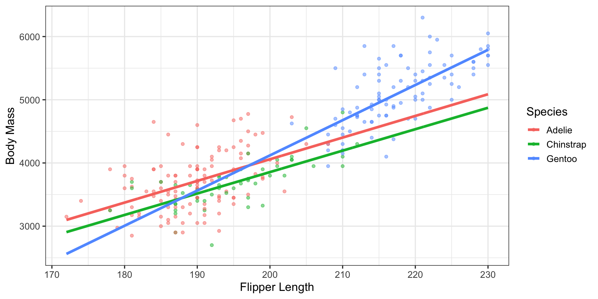
Note that our new model, including the interaction between species and year includes nine (9) parallel lines

Additional Flexibility with Interactions
Note that our new model, including the interaction between species and year includes nine (9) parallel lines
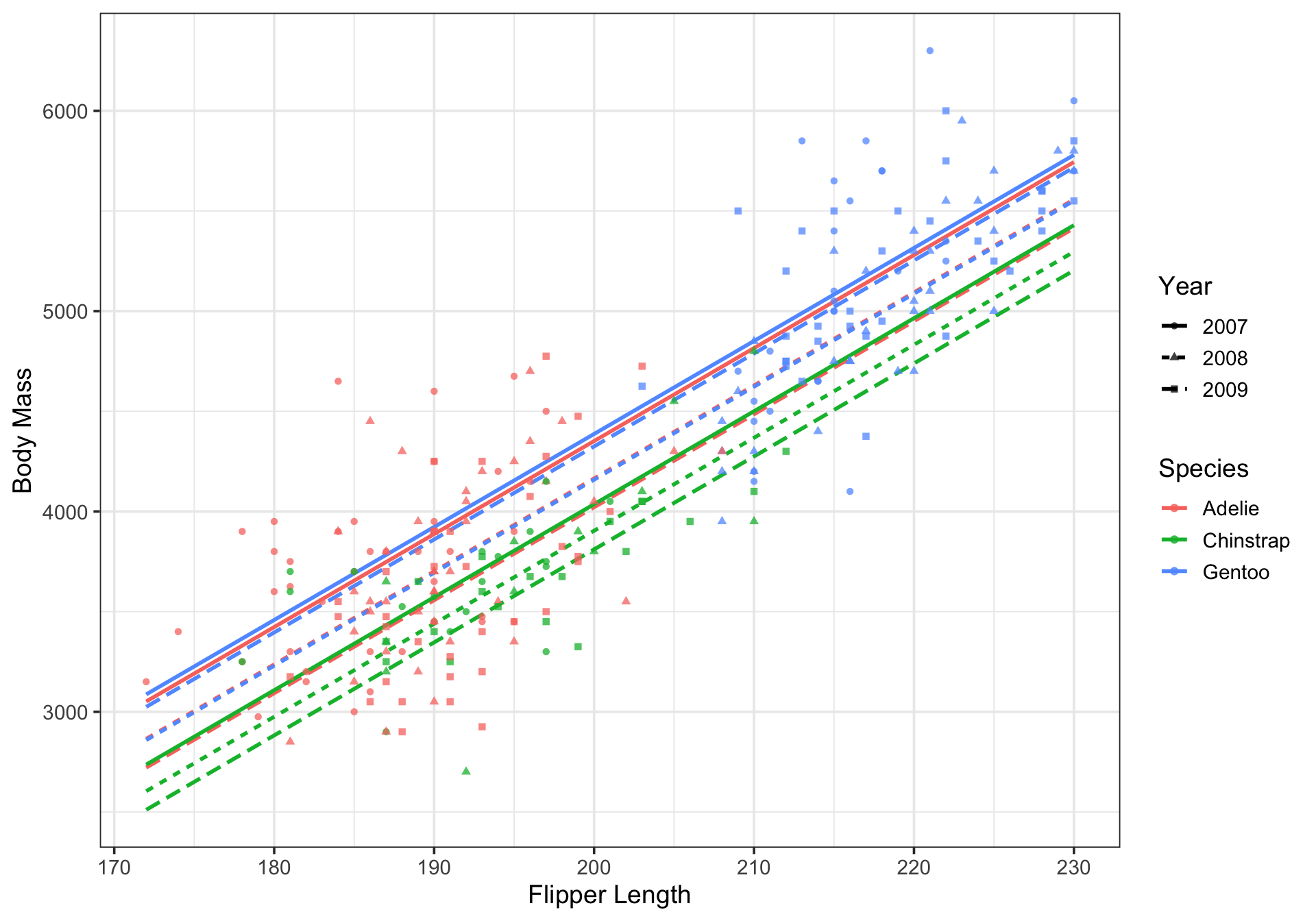
Where our model including species and year independently only included six
Additional Flexibility with Interactions
\(\bigstar\) Let’s try it! \(\bigstar\)
- Whether you plotted your model predictions or not, how many parallel lines does your interaction model consist of?
- How many additional \(\beta\)-coefficients were estimated for your interaction model, compared to the number of \(\beta\)-coefficients that would have been estimated for a model with the same predictors but no interaction?
Mini-Summary: Interactions Between Categorical Variables
Interactions between pairs of categorical variables can be used to investigate whether the effect of a change in levels of one of the variables depends on the level of the second categorical variable
The result of including such an interaction is a unique model intercept for each combination of levels of the categorical variables
Note that the resulting models will still be parallel unless different types of interactions are also present in the model
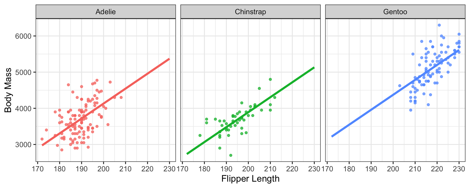
Interactions Between a Categorical Predictor and a Numerical Predictor
Another reasonable question to ask is whether the association between flipper length and body mass changes based on the species of penguin
We can investigate this by constructing and analysing a model that includes an interaction between species and flipper length
Again, we can compare the model forms below:
Model with Flipper Length and Species Independently:
\[\mathbb{E}\left[\text{body mass}\right] = \beta_0 + \beta_1\cdot\left(\text{flipper length}\right) + \beta_2\cdot\left(\text{speciesChinstrap}\right) + \beta_3\cdot\left(\text{speciesGentoo}\right)\]
Model with Interaction Between Flipper Length and Species:
\[\begin{align}\mathbb{E}\left[\text{body mass}\right] = \beta_0 + &\beta_1\cdot\left(\text{flipper length}\right) + \beta_2\cdot\left(\text{speciesChinstrap}\right) + \beta_3\cdot\left(\text{speciesGentoo}\right) + \\ &\beta_4\cdot\left(\text{flipper length}\right)\left(\text{speciesChinstrap}\right) +\\ &\beta_5\cdot\left(\text{flipper length}\right)\left(\text{speciesGentoo}\right) \end{align}\]
Building the Model
We construct our model in the same way as we did with the previous interaction model
mlr_fls_isfl_spec <- linear_reg() %>%
  set_engine("lm")

mlr_fls_isfl_rec <- recipe(body_mass_g ~ flipper_length_mm + species,
                           data = penguins_train) %>%
  step_dummy(species) %>%
  step_interact(~ starts_with("species"):flipper_length_mm)

mlr_fls_isfl_wf <- workflow() %>%
  add_model(mlr_fls_isfl_spec) %>%
  add_recipe(mlr_fls_isfl_rec)

mlr_fls_isfl_fit <- mlr_fls_isfl_wf %>%
  fit(penguins_train)
Building the Model
\(\bigstar\) Let’s try it! \(\bigstar\)
- Drop one of your categorical predictors from your earlier model (if you’d like), and consider a model with just one numerical and one categorical predictor
- Create a model specification and recipe that will accommodate an interaction between your numerical and categorical predictor (only one of them, even if your model has multiple…just to keep things relatively “simple”)
- Package your specification and recipe together into a workflow
- Fit your workflow to your training data
The Estimated Model
| term | estimate | std.error | statistic | p.value |
|---|---|---|---|---|
| (Intercept) | -2797.759952 | 1059.375697 | -2.6409516 | 0.0087881 |
| flipper_length_mm | 34.282823 | 5.582906 | 6.1406767 | 0.0000000 |
| species_Chinstrap | -129.708846 | 1708.747729 | -0.0759087 | 0.9395524 |
| species_Gentoo | -4216.630301 | 1702.555778 | -2.4766474 | 0.0139247 |
| species_Chinstrap_x_flipper_length_mm | -0.366684 | 8.853089 | -0.0414188 | 0.9669951 |
| species_Gentoo_x_flipper_length_mm | 21.389349 | 8.284884 | 2.5817319 | 0.0104008 |
\(\displaystyle{\mathbb{E}\left[\text{body mass}\right] \approx ...}\)
The Estimated Model (Cont’d.)
The Estimated Model
\(\bigstar\) Let’s try it! \(\bigstar\)
- As with the model you built previously, extract the estimated model from the fitted object
- Write down the estimated model
- If you would like, try to plot the model
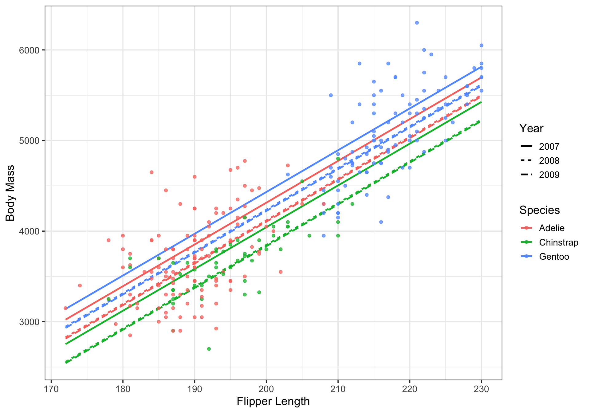
Additional Flexibility with Interactions
Note that our new model, including an interaction between species and flipper length still includes only three lines
Those lines are no longer parallel, though
We needed additional \(\beta\)-coefficients to accommodate our slope adjustments
\(\bigstar\) How many additional \(\beta\)-coefficients did your most recent interaction model require?
Interpreting this Interaction Model
Overarching Model:
\[\begin{align}\mathbb{E}\left[\text{body mass}\right] = -2797.76 ~+~ &34.28\cdot\left(\text{flipper length}\right) - 129.71\cdot\left(\text{speciesChinstrap}\right) +\\ &- 4216.63\cdot\left(\text{speciesGentoo}\right) +\\ &- 0.37\cdot\left(\text{flipper length}\right)\left(\text{speciesChinstrap}\right) +\\ &21.39\cdot\left(\text{flipper length}\right)\left(\text{speciesGentoo}\right) \end{align}\]
Model for Adelie Penguins:
\[\begin{align}\mathbb{E}\left[\text{body mass}\right] = -2797.76 ~+~ &34.28\cdot\left(\text{flipper length}\right) \end{align}\]
Given an Adelie penguin, an increase of 1mm in flipper length is associated with an increase in expected body mass by about 34.28g
Interpreting this Interaction Model
Overarching Model:
\[\begin{align}\mathbb{E}\left[\text{body mass}\right] = -2797.76 ~+~ &34.28\cdot\left(\text{flipper length}\right) - 129.71\cdot\left(\text{speciesChinstrap}\right) +\\ &- 4216.63\cdot\left(\text{speciesGentoo}\right) +\\ &- 0.37\cdot\left(\text{flipper length}\right)\left(\text{speciesChinstrap}\right) +\\ &21.39\cdot\left(\text{flipper length}\right)\left(\text{speciesGentoo}\right) \end{align}\]
Model for Chinstrap Penguins:
\[\begin{align}\mathbb{E}\left[\text{body mass}\right] = -2927.47 ~+~ &33.91\cdot\left(\text{flipper length}\right) \end{align}\]
Given a Chinstrap penguin, an increase of 1mm in flipper length is associated with an increase in expected body mass by about 33.91g
Note that this is not significantly different than the expected change for Adelies
Interpreting this Interaction Model
Overarching Model:
\[\begin{align}\mathbb{E}\left[\text{body mass}\right] = -2797.76 ~+~ &34.28\cdot\left(\text{flipper length}\right) - 129.71\cdot\left(\text{speciesChinstrap}\right) +\\ &- 4216.63\cdot\left(\text{speciesGentoo}\right) +\\ &- 0.37\cdot\left(\text{flipper length}\right)\left(\text{speciesChinstrap}\right) +\\ &21.39\cdot\left(\text{flipper length}\right)\left(\text{speciesGentoo}\right) \end{align}\]
Model for Gentoo Penguins:
\[\begin{align}\mathbb{E}\left[\text{body mass}\right] = -7014.39 ~+~ &55.67\cdot\left(\text{flipper length}\right) \end{align}\]
Given a Gentoo penguin, an increase of 1mm in flipper length is associated with an increase in expected body mass by about 55.67g
Interpreting Models with Categorical-Numerical Interactions
\(\bigstar\) Let’s try it! \(\bigstar\)
- Provide interpretations for your interaction model with respect to at least two of the levels of the categorical variable involved in your interaction
Mini-Summary: Interactions Between a Categorical and a Numerical Variable
- Interactions between a categorical variable and a numerical variable can be used to investigate whether the effect of a unit increase in the numerical variable differs across the levels of the categorical variable
- The result of including such an interaction is a unique model slope(\(^*\)) for each level of the categorical variable
Interactions Between Numerical Variables
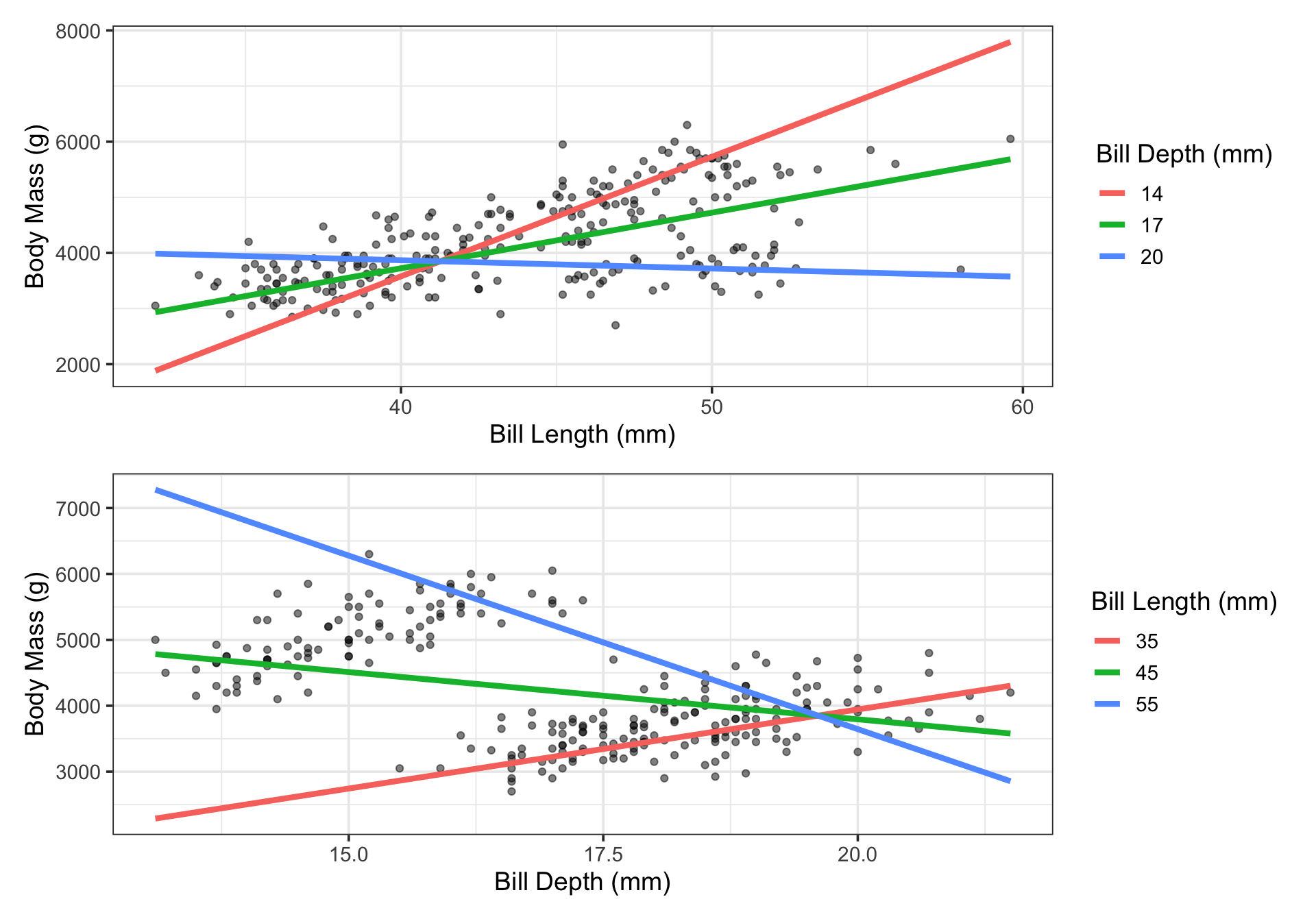
Also reasonable, yet more difficult to interpret, is the possibility that the association between bill length and penguin body mass is dependent on the penguin’s bill depth (another numerical predictor)
We’ve switched from flipper length to bill length and bill depth because some interaction between those features is intuitively plausible
We can investigate whether such an interaction effect is present by constructing and analysing a model which includes an interaction term between bill length and bill depth
As we did previously, we can compare the proposed model forms:
Model with Bill Length and Bill Depth Independently:
\[\begin{align}\mathbb{E}\left[\text{body mass}\right] = \beta_0 +~ &\beta_1 \cdot\left(\text{bill length}\right) + \beta_2\cdot\left(\text{bill depth}\right) \end{align}\]
Model with Interaction Between Bill Length and Bill Depth:
\[\begin{align} \mathbb{E}\left[\text{body mass}\right] = \beta_0 +~ &\beta_1 \cdot\left(\text{bill length}\right) + \beta_2\cdot\left(\text{bill depth}\right) +\\ &\beta_3\cdot\left(\text{bill length}\right)\left(\text{bill depth}\right) \end{align}\]
Building the Model
No real changes here – we’ll use step_interact() again
mlr_blbd_i_spec <- linear_reg() %>%
  set_engine("lm")

mlr_blbd_i_rec <- recipe(body_mass_g ~ bill_length_mm + bill_depth_mm,
                           data = penguins_train) %>%
  step_interact(~ bill_length_mm:bill_depth_mm)

mlr_blbd_i_wf <- workflow() %>%
  add_model(mlr_blbd_i_spec) %>%
  add_recipe(mlr_blbd_i_rec)

mlr_blbd_i_fit <- mlr_blbd_i_wf %>%
  fit(penguins_train)
Building the Model
\(\bigstar\) Let’s try it! \(\bigstar\)
- Choose two numerical predictors of price which might have an interaction effect in determining price of the rentals in your data set
- As with the previous models, define the model specification and recipe, then build and fit the workflow to your training data
The Estimated Model
| term | estimate | std.error | statistic | p.value |
|---|---|---|---|---|
| (Intercept) | -27159.5171 | 3343.877732 | -8.122162 | 0 |
| bill_length_mm | 751.5601 | 73.587759 | 10.213112 | 0 |
| bill_depth_mm | 1581.3298 | 188.042339 | 8.409435 | 0 |
| bill_length_mm_x_bill_depth_mm | -38.3255 | 4.155655 | -9.222491 | 0 |
\(\displaystyle{\mathbb{E}\left[\text{body mass}\right] = \cdots}\)
The Estimated Model (Cont’d.)
The Estimated Model
\(\bigstar\) Let’s try it! \(\bigstar\)
- Extract the estimated model from the fitted object
- Write down the equation for your estimated model
- Construct a plot, if you would like to do so
Additional Flexibility with Interactions
This model consists of a warped surface.
As long as we fix a value of bill length, then the expected effect of a unit increase in bill depth on penguin body mass is constant
Similarly, as long as we fix a value of bill depth, then the expected effect of a unit increase in bill length on penguin body mass is constant
The effect of a unit increase in either bill length or depth, however, depends on the current level of the other predictor
\(\bigstar\) How many additional \(\beta\)-coefficients were required for your newest interaction model?
Interpreting this Interaction Model
As a reminder, the general form for this interaction model was
\[\begin{align} \mathbb{E}\left[\text{body mass}\right] = \beta_0 +~ &\beta_1 \cdot\left(\text{bill length}\right) + \beta_2\cdot\left(\text{bill depth}\right) +\\ &\beta_3\cdot\left(\text{bill length}\right)\left(\text{bill depth}\right) \end{align}\]
Effect of a Unit Change in Bill Length, Holding Bill Depth Constant:
Holding bill depth constant, a unit increase in bill length is associated with an expected increase in penguin body mass of \(\displaystyle{\beta_1 + \beta_3\cdot\left(\text{bill depth}\right)}\)
Effect of a Unit Change in Bill Depth, Holding Bill Length Constant:
Holding bill length constant, a unit increase in bill depth is associated with an expected increase in penguin body mass of \(\displaystyle{\beta_2 + \beta_3\cdot\left(\text{bill length}\right)}\)
Interpreting this Interaction Model
Our estimated model was
\[\begin{align} \mathbb{E}\left[\text{body mass}\right] = -27159.52 +~ &751.56 \cdot\left(\text{bill length}\right) + 1581.33\cdot\left(\text{bill depth}\right) +\\ &-38.33\cdot\left(\text{bill length}\right)\left(\text{bill depth}\right) \end{align}\]
Effect of a Unit Change in Bill Length, Holding Bill Depth Constant:
Holding bill depth constant, a unit increase in bill length is associated with an expected increase in penguin body mass of \(\displaystyle{\beta_1 + \beta_3\cdot\left(\text{bill depth}\right)}\)
For this particular estimated model,
\[\begin{align} \beta_1 + \beta_3 \cdot\left(\text{bill depth}\right) &\approx 751.56 - 38.33\cdot\left(\text{bill depth}\right) \end{align}\]
For Example: Holding bill depth constant at 15mm, a unit increase in bill length is associated with an expected increase in body mass by about \[\begin{align} 751.56 - 38.33\cdot\left(15\right) &= 176.61\text{g} \end{align}\]
Interpreting this Interaction Model
Our estimated model was
\[\begin{align} \mathbb{E}\left[\text{body mass}\right] = -27159.52 +~ &751.56 \cdot\left(\text{bill length}\right) + 1581.33\cdot\left(\text{bill depth}\right) +\\ &-38.33\cdot\left(\text{bill length}\right)\left(\text{bill depth}\right) \end{align}\]
Effect of a Unit Change in Bill Depth, Holding Bill Length Constant:
Holding bill length constant, a unit increase in bill depth is associated with an expected increase in penguin body mass of \(\displaystyle{\beta_2 + \beta_3\cdot\left(\text{bill length}\right)}\)
For this particular estimated model,
\[\begin{align} \beta_1 + \beta_3 \cdot\left(\text{bill depth}\right) &\approx 1581.33 - 38.33\cdot\left(\text{bill length}\right) \end{align}\]
For Example: Holding bill length constant at 40mm, a unit increase in bill depth is associated with an expected increase in body mass by about \[\begin{align} 1581.33 - 38.33\cdot\left(40\right) &= 48.13\text{g} \end{align}\]
Interpreting Models with Numerical-Numerical Interactions
\(\bigstar\) Let’s try it! \(\bigstar\)
- Provide interpretations of the association between each of your numerical predictors and the response under this newest interaction model
Mini-Summary: Interactions Between Two Numerical Variables
- Interactions between two numerical variables can be used to investigate whether the effect of a unit increase in one numerical predictor depends on the level of the other
- The result of including such an interaction is a warped surface such that a cross-section holding one of the numerical predictors constant results in a straight line (constant slope) relationship between the remaining numerical predictor and the response
Summary
Interaction terms are another example of higher-order terms in models that allow us to model associations more complex than “straight line”
We add interaction terms to a model using the
{tidymodels}framework by appendingstep_interact()to our recipestep_interact()requires a tilde~followed by the interaction variables with a colon separating them- There are three types of two-way interaction (categorical-categorical, categorical-numerical, numerical-numerical)
Categorical-categorical interactions result in additional **intercept adjustments* corresponding to each combination of levels of the interacting predictors
Categorical-numerical interactions result in slope adjustments between the numerical predictor and response for each level of the categorical predictor
Numerical-numerical interactions result in a warped prediction surface such that the “slopes” in the direction of each numerical predictor change, however, if we look at a cross-section holding one of the numerical predictors constant, then the slope in the direction of the other numerical predictor is constant(\(^*\))
As we mentioned last time, interpreting models with higher-order terms can be a complex business, requiring some calculus knowledge – we’ll get some help from the
{marginaleffects}package next
Wait…What About Interactions Between More than Two Predictors???
Sup. It's a dirty job, but someone's gotta provide plausible and defensible rationales for nonmonotonic interactions. pic.twitter.com/arCeYeK9Ot
— Research Wahlberg (@ResearchMark) October 29, 2014
Next Time…
Model Inference and Interpreation with the {marginaleffects} Package