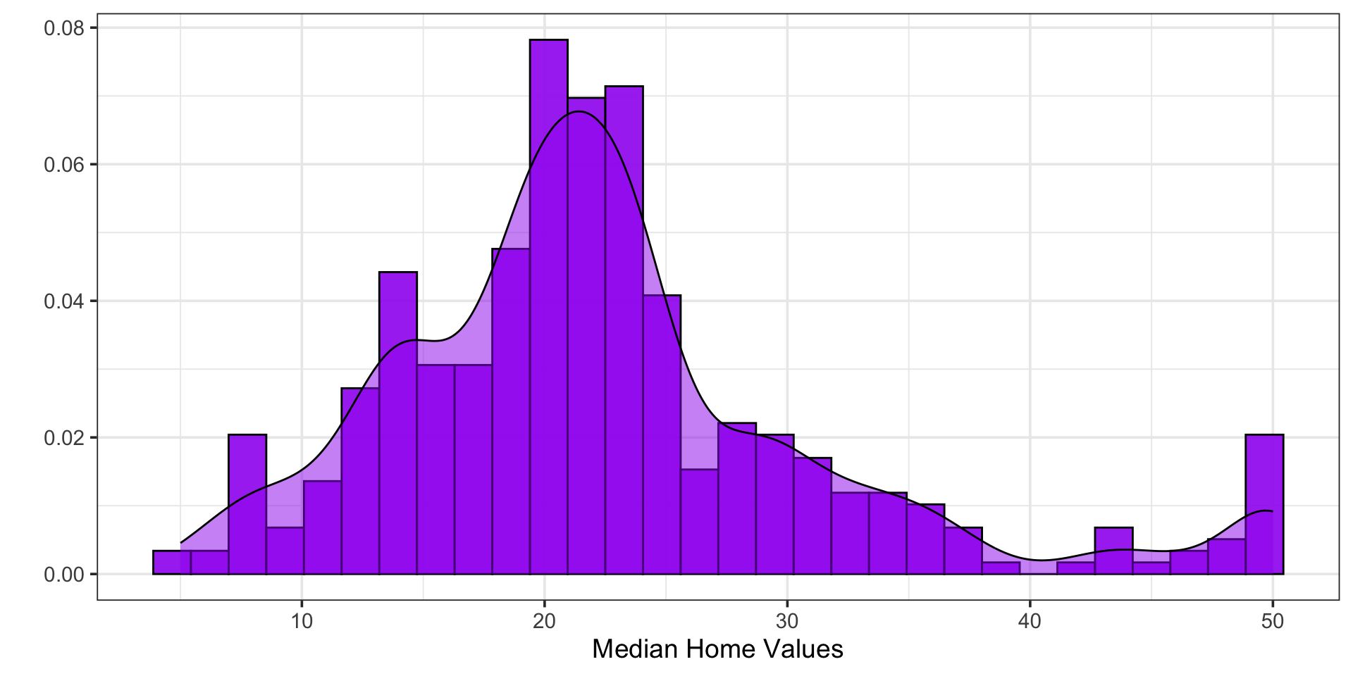
This Boston housing dataset is quite famous (and problematic), and includes features on each neighborhood and the corresponding median home value in that neighborhood. You can see a data dictionary here. The data set has many interesting features and even allows us some ability to explore structural racism in property valuation in 1970s Boston.
boston <-read_csv("https://raw.githubusercontent.com/selva86/datasets/master/BostonHousing.csv" )boston %>%head()
choose at least one of the available numeric predictors to include in polynomial terms
create an instance of a linear regression model specification
create a recipe and append step_poly() to it in order to create the higher-order terms
package your model specification and recipe together into a workflow
Fit and Assess Model
Fit the Model to Training Data:
mlr_me_fit <- mlr_me_wf %>%fit(boston_train)
Global Model Utility:
mlr_me_fit %>%glance()
r.squared
adj.r.squared
sigma
statistic
p.value
df
logLik
AIC
BIC
deviance
df.residual
nobs
0.703557
0.6995832
5.055401
177.0504
0
5
-1148.907
2311.814
2339.377
9532.791
373
379
Individual Term-Based Assessments:
mlr_me_fit %>%extract_fit_engine() %>%tidy()
term
estimate
std.error
statistic
p.value
(Intercept)
39.8979924
1.3882165
28.7404684
0.0000000
chas
4.9606104
1.0056444
4.9327680
0.0000012
age_poly_1
0.0975669
0.0506654
1.9257113
0.0549003
age_poly_2
-0.0002641
0.0004208
-0.6277625
0.5305437
lstat_poly_1
-2.6383538
0.1457957
-18.0962367
0.0000000
lstat_poly_2
0.0482353
0.0041368
11.6600251
0.0000000
Drop the Curvi-linear Term for age
mlr_me_rec <-recipe(medv ~ age + lstat + chas, data = boston_train) %>%step_poly(lstat, degree =2, options =list(raw =TRUE))mlr_me_wf <-workflow() %>%add_model(mlr_me_spec) %>%add_recipe(mlr_me_rec)
Re-Fit the Model to Training Data:
mlr_me_fit <- mlr_me_wf %>%fit(boston_train)
Assess Updated Model
Global Model Utility:
mlr_me_fit %>%glance()
r.squared
adj.r.squared
sigma
statistic
p.value
df
logLik
AIC
BIC
deviance
df.residual
nobs
0.7032438
0.7000699
5.051304
221.5734
0
4
-1149.107
2310.214
2333.839
9542.862
374
379
Individual Term-Based Assessments:
mlr_me_fit %>%extract_fit_engine() %>%tidy()
term
estimate
std.error
statistic
p.value
(Intercept)
40.5405112
0.9370994
43.261697
0.0000000
age
0.0666784
0.0120705
5.524075
0.0000001
chas
4.9657731
1.0047958
4.942072
0.0000012
lstat_poly_1
-2.6277451
0.1446957
-18.160497
0.0000000
lstat_poly_2
0.0477036
0.0040459
11.790647
0.0000000
A Note on Higher-Order Terms and Significance
If a higher-order term in a model is statistically significant, then all lower-order components of that term must be kept in the model
For example, if a term for age\(\cdot\)lstat\(^2\) is included in a model, then each of the following terms must be kept regardless of statistical significance
age
lstat
age\(\cdot\)lstat
lstat\(^2\)
Fitting, Assessing, and Updating the Model (🔁)
\(\bigstar\) Let’s try it! \(\bigstar\)
Again, if you are playing along with your Air BnB data…
fit your model workflow to your training data
conduct both global and term-based model assessments
reduce, refit, and reassess your model as needed
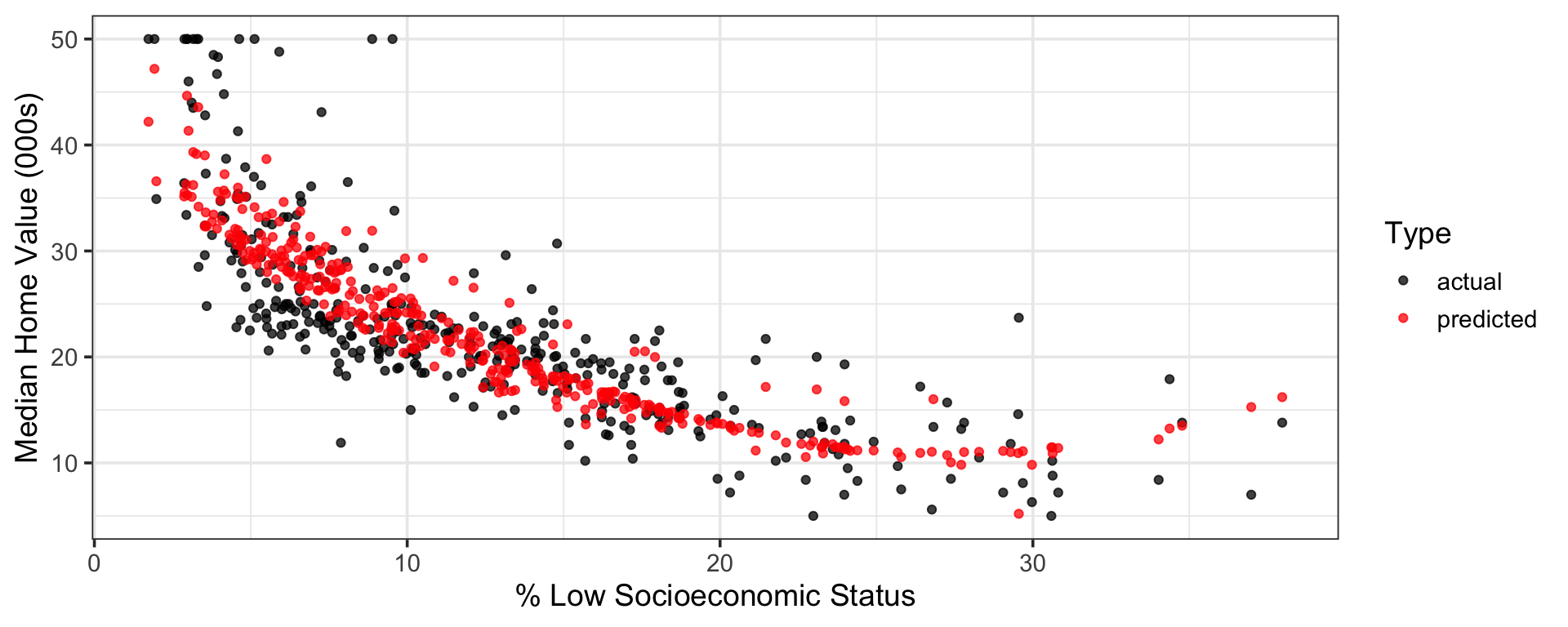
Visualizing Model Predictions [Training Data]
Code
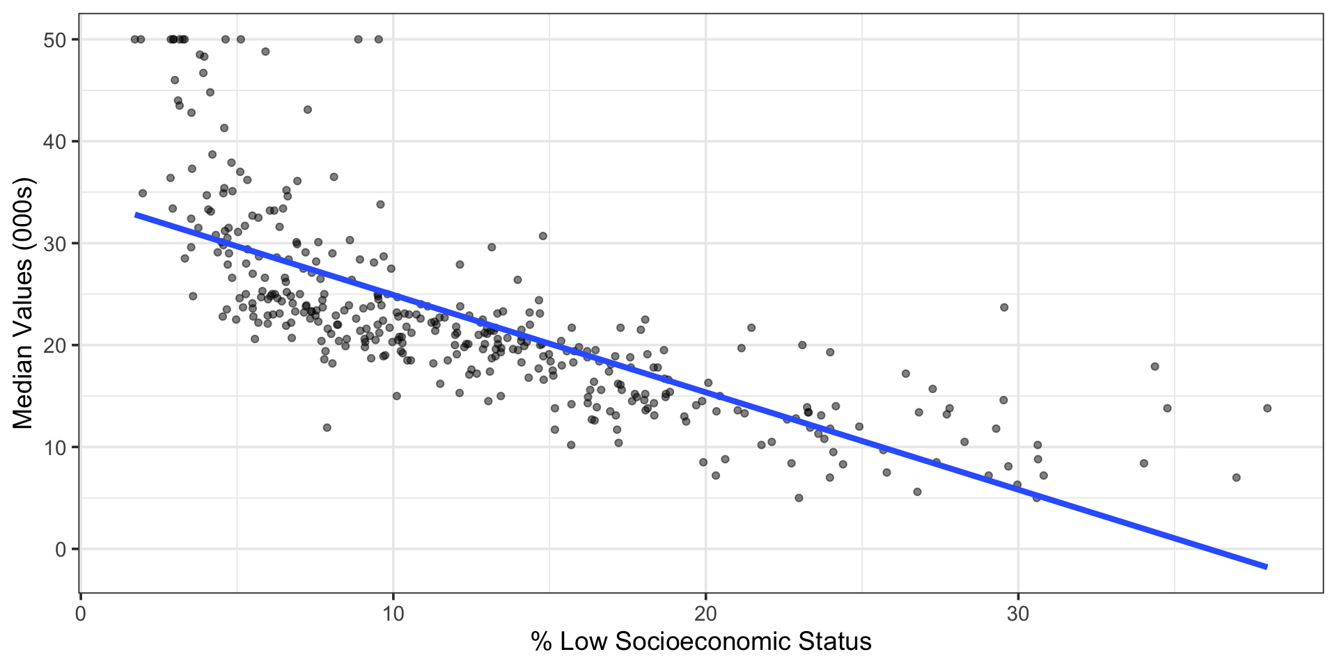
point_colors <-c("actual"="black", "predicted"="red")mlr_me_fit %>%augment(boston_train) %>%ggplot() +geom_point(aes(x = lstat, y = medv, color = actual),alpha =0.75) +geom_point(aes(x = lstat, y = .pred, color = predicted), alpha =0.75) +scale_color_manual(values = point_colors) +labs(x ="% Low Socioeconomic Status",y ="Median Home Value (000s)",color ="Type")
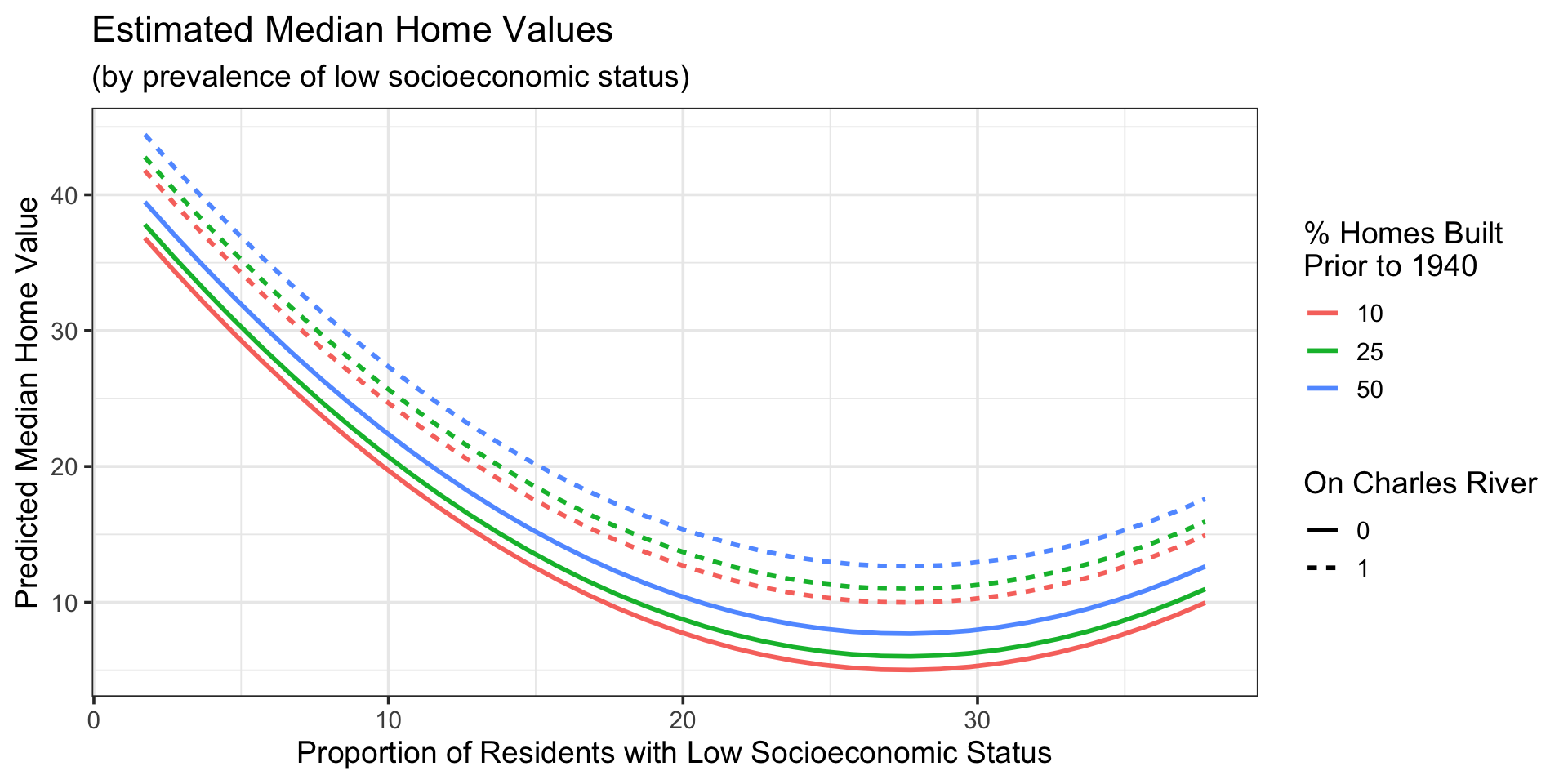
Model At Various Age Thresholds
Code
new_data <-crossing(age =c(10, 25, 50),chas =c(0, 1),lstat =seq(min(boston_train$lstat, na.rm =TRUE),max(boston_train$lstat, na.rm =TRUE),length.out =250))mlr_me_fit %>%augment(new_data) %>%ggplot() +geom_line(aes(x = lstat, y = .pred, color =as.factor(age),linetype =as.factor(chas)),lwd =1) +labs(x ="Proportion of Residents with Low Socioeconomic Status",y ="Predicted Median Home Value",title ="Estimated Median Home Values",subtitle ="(by prevalence of low socioeconomic status)",color ="% Homes Built \nPrior to 1940",linetype ="On Charles River")
The model consists of curved surfaces
One surface for when the neighborhood is on the Charles River, and another for neighborhoods off of it
The cross-sections for each surface at different age thresholds are parallel
Visualizing Model Predictions
\(\bigstar\) Let’s try it! \(\bigstar\)
For those still following along with the Air BnB data…
plot your model’s fitted values along with the observed rental prices for your training data
plot of your model’s predictions in relation to a predictor that has a higher-order term in your model – vary the values of the other significant predictors across different thresholds to visualize their effect, as in the previous slide
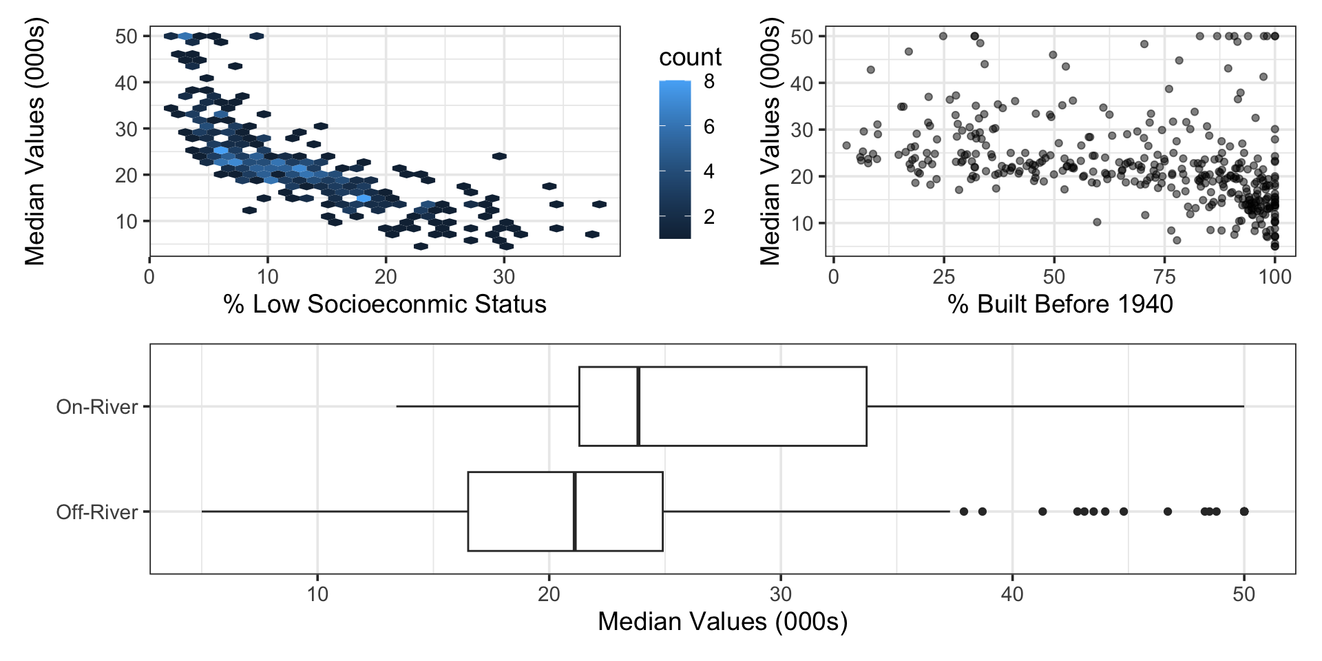
(Intercept) The expected median home value for a neighborhood with 0% of residents being of low socioeconomic status, 0% of homes built before 1940, and being away from the Charles River is about $40,541
(age) Holding location relative to the Charles River and percentage of residents with low socioeconomic status constant, a one percentage-point increase in the proportion of homes built prior to 1940 is associated with an expected increase of about $67 in median home value
(chas) Holding percentage of residents with low socioeconomic status and percentage of homes built before 1940 constant, a neighborhood on the Charles River is expected to have higher median home values by about $4,966
The association between lstat and median home values is not constant!
The expected change in median home values due to a change in the percentage of residents with low socioeconomic status depends on the “current” percentage.
(lstat) Holding the location of a neighborhood relative to the Charles River and the percentage of homes built before 1940, a one percentage-point increase in the percentage of residents of low socioeconomic status is expected to be associated with a change in median home values of about
\[-2.628 + 2\cdot\left(0.048\right)\cdot\left(\text{lstat}\right)~~~~~~~~\left(\text{times 1000 to convert to thousands}\right)\]
(lstat) Holding the location of a neighborhood relative to the Charles River and the percentage of homes built before 1940, a one percentage-point increase in the percentage of residents of low socioeconomic status is expected to be associated with a change in median home values of about
\[-2.628 + 2\left(0.048\right)\cdot\left(\text{lstat}\right)~~~~~~~~\left(\text{times 1000 to convert to thousands}\right)\]
For Example: If the current percentage of residents of low socioeconomic status is 10%, then holding location relative to the Charles River and the percentage of homes build before 1940 constant, an increase to 11% of residents with low socioeconomic status is expected to be associated with a change in median home values by about
Similarly, if the current percentage was 33%, then we would expect an increase of about $540 in a similar neighborhood but where the percentage of residents of low socioeconomic status is 34%
where the only two terms involving the predictor \(x\) are the ones shown.
Interpretation of a Unit Increase in \(x\): Holding all other predictors constant, a unit increase in \(x\) is associated with an expected change in the response by about \(\beta_1 + 2\cdot\beta_2\cdot x\).
A Bit of Calculus: Those of you with a Calculus background will recognize this as the partial derivative of the model with respect to \(x\).
Taking the partial derivative is how you examine the effect of a change in any numerical variable on the response.
Two class meetings from now, we’ll see how we can use the {marginaleffects} package to make our interpretations easier, especially for those of you without a calculus background.
Interpreting your Model
\(\bigstar\) Let’s try it! \(\bigstar\)
If you have a model that predicts prices of Air BnB rentals…
provide interpretations of the intercept (if relevant) and the association between each surviving predictor and the response
Summary
We can use higher order terms to model associations that are more complex than “straight line”
Higher order terms include polynomial terms (a predictor to a positive integer power) and interaction terms (a product of two or more predictors)
We add polynomial terms to a model using the {tidymodels} framework by appending step_poly() to our recipe
Models with polynomial terms approximate curved relationships between the predictor and response
We use the degree argument of step_poly() to determine the degree of the polynomial term (higher degree means more wiggly, and more \(\beta\)-coefficients)
Setting options = list(raw = TRUE) within step_poly() prevents the function from attempting to build “orthogonal polynomial terms” which would reduce interpretability
To interpret models with higher-order terms, we’ll need a bit of calculus (or help from a package like {marginaleffects})
If a model \(\mathbb{E}\left[y\right] = \beta_0 + \beta_1 x + \beta_2 x^2 + \cdots\) includes a second degree term for the predictor \(x\) and \(x\) is not included in any model terms other than those shown, the effect of a unit increase in \(x\) on the response \(y\) is an increase of about \(\beta_1 + 2\beta_2 x\)