Inclusion and Interpretation of Catgorical Predictors in Linear Regression Models

Dr. Gilbert

October 11, 2024

Motivation

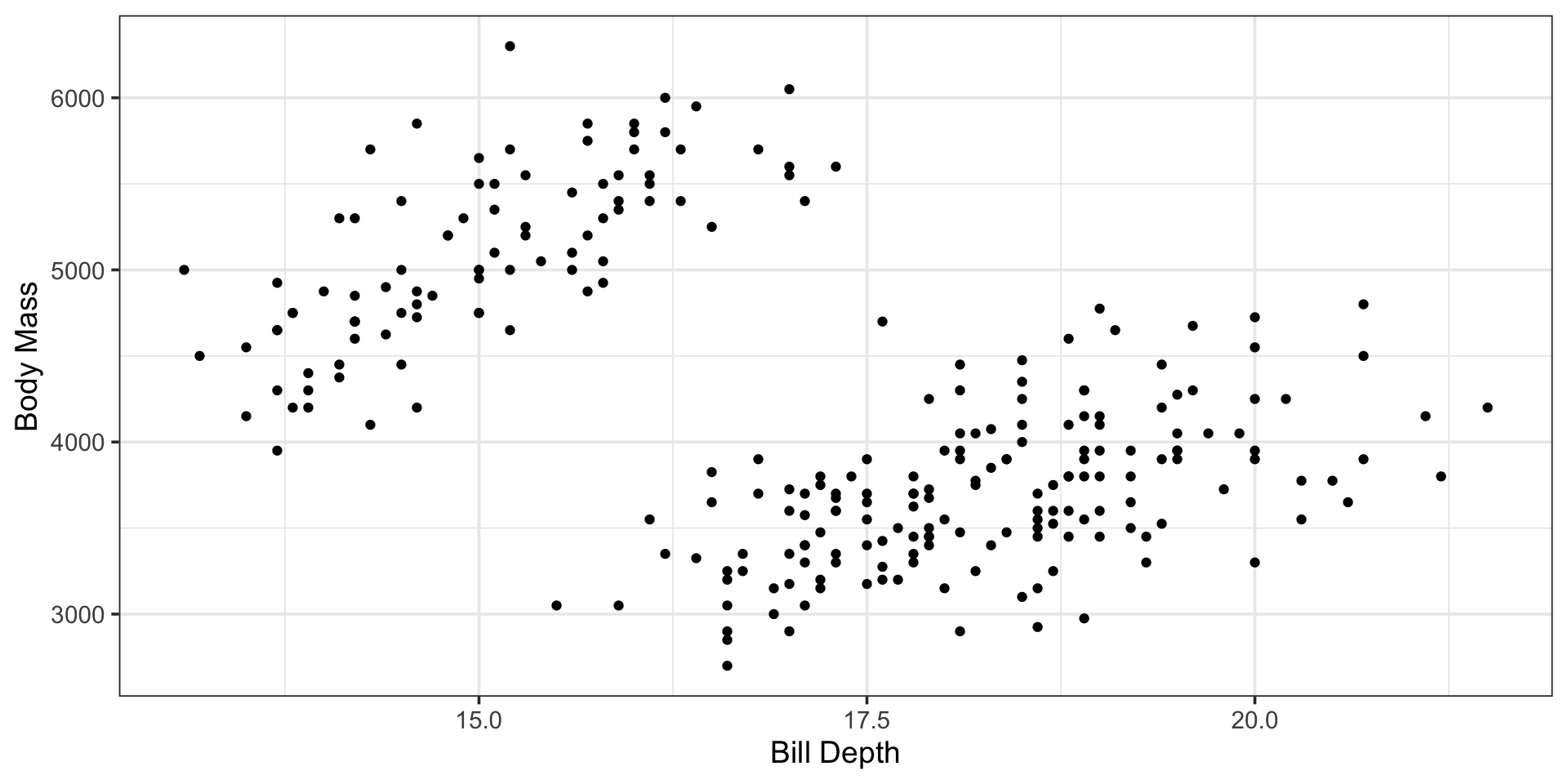
Motivation

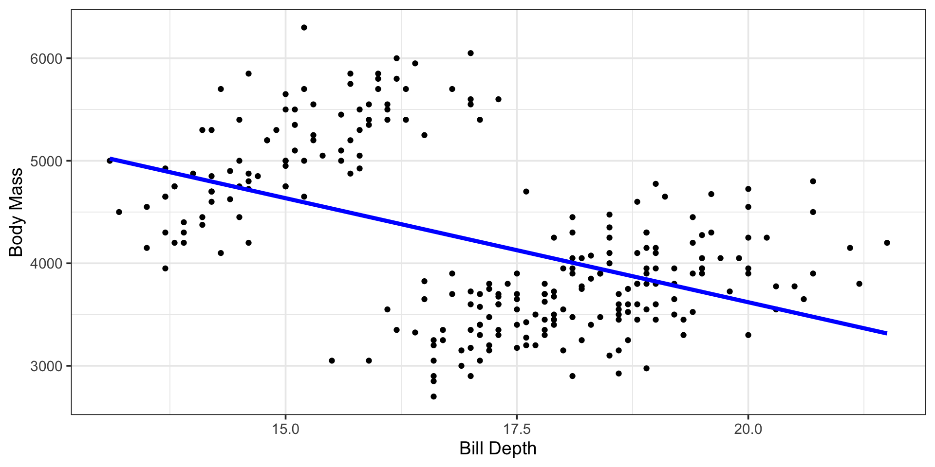
r.squared	adj.r.squared	sigma	statistic	p.value	df	logLik	AIC	BIC	deviance	df.residual	nobs
0.2260831	0.2230361	723.2657	74.2006	0	1	-2047.691	4101.382	4112.018	132870759	254	256

term	estimate	std.error	statistic	p.value
(Intercept)	7679.4255	406.12272	18.909126	0
bill_depth_mm	-202.9711	23.56299	-8.613977	0

Motivation

The Highlights

• ANOVA as a linear regression model

• Strategies for using categorical predictors in a model

  • Ordinal scorings
  • One-hot encodings versus dummy encodings

• Feature engineering steps in recipes

• Handling unknown or novel levels of a categorical variable

• Fitting a model with categorical and numerical variables

• Interpreting models with categorical predictors

Playing Along

As always, you are encouraged to implement the ideas and techniques discussed here with your own data. You should…

1. Open RStudio and ensure that you are working within your MAT300 project space
2. Open the notebook which includes your models for Air BnB rentals
3. Run all of the code in that notebook

You’ll add to that notebook here

ANalysis Of VAriance

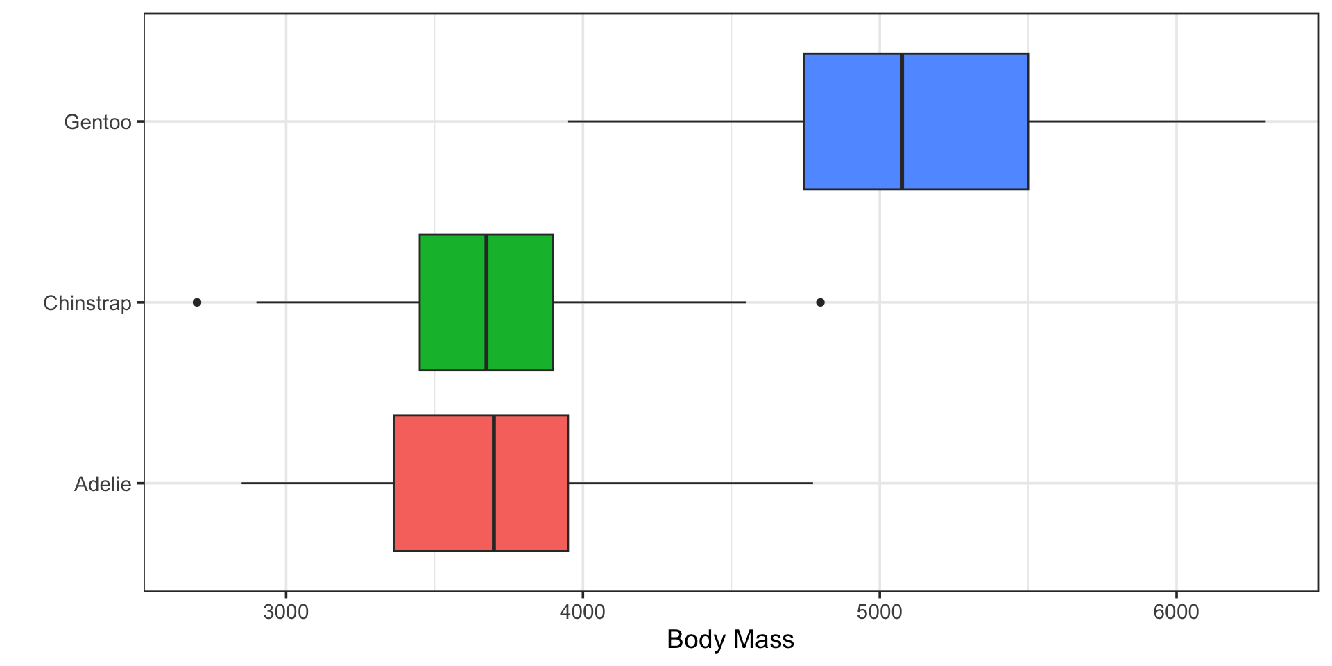
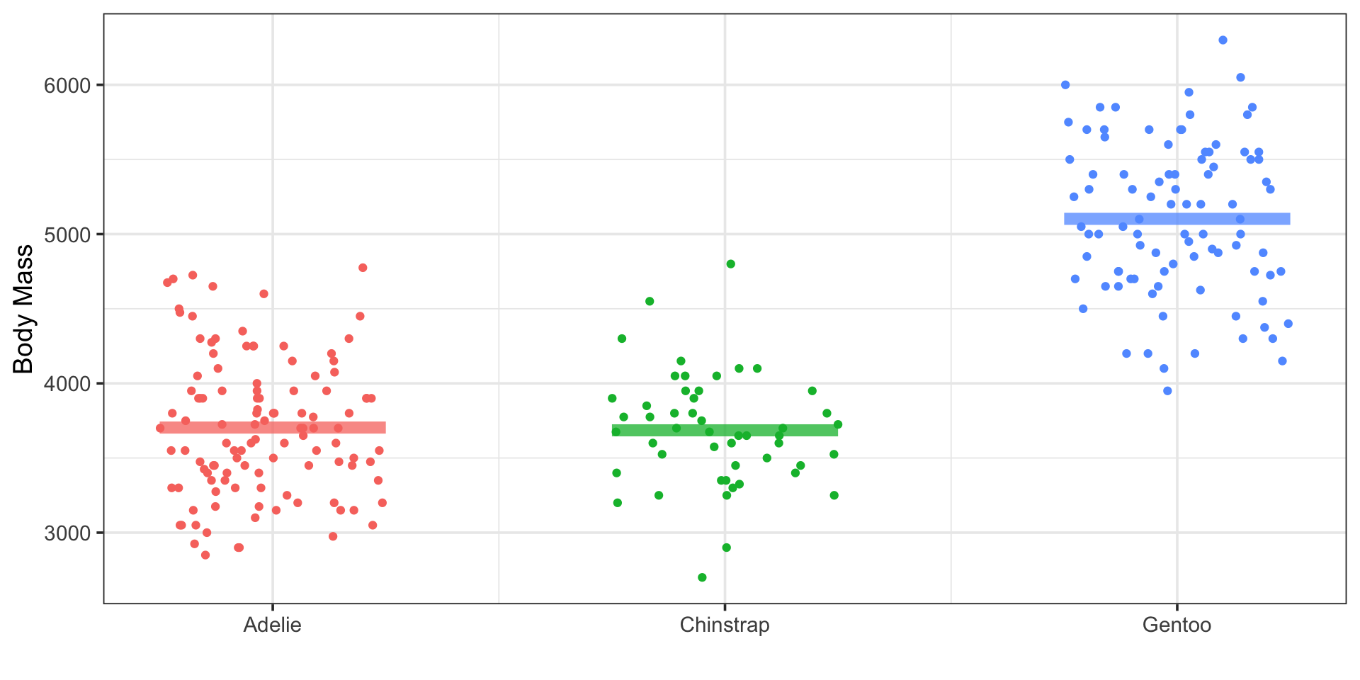
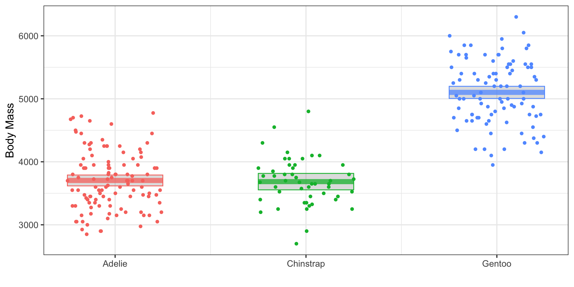
Does penguin body mass vary by species?

\[\begin{array}{lcl} H_0 & : & \mu_{\text{Adelie}} = \mu_{\text{Chinstrap}} = \mu_{\text{Gentoo}}\\ H_a & : & \text{At least one species has different average body mass}\end{array}\]

ANalysis Of VAriance

Does penguin body mass vary by species?

\[\begin{array}{lcl} H_0 & : & \mu_{\text{Adelie}} = \mu_{\text{Chinstrap}} = \mu_{\text{Gentoo}}\\ H_a & : & \text{At least one species has different average body mass}\end{array}\]

ANOVA Test:

ANOVAtable <- aov(body_mass_g ~ species, data = penguins_train)

ANOVAtable %>%
  tidy()

term	df	sumsq	meansq	statistic	p.value
species	2	116165670	58082835.2	264.6767	0
Residuals	253	55520401	219448.2	NA	NA

ANalysis Of VAriance as Linear Regression

Does penguin body mass vary by species?

\[\mathbb{E}\left[\text{body mass}\right] = \beta_0 + \beta_1\cdot\left(\text{???}\right)\]

Model-Based Test:

r.squared	adj.r.squared	sigma	statistic	p.value	df	logLik	AIC	BIC	deviance	df.residual	nobs
0.6766167	0.6740604	468.453	264.6767	0	2	-1935.995	3879.99	3894.171	55520401	253	256

term	estimate	std.error	statistic	p.value
(Intercept)	3703.94737	43.87464	84.4211365	0.0000000
species_Chinstrap	-18.44737	79.46036	-0.2321581	0.8166029
species_Gentoo	1398.22654	65.65281	21.2972846	0.0000000

ANalysis Of VAriance as Linear Regression

Does penguin body mass vary by species?

\[\mathbb{E}\left[\text{body mass}\right] = \beta_0 + \beta_1\cdot\left(\text{speciesChinstrap}\right) + \beta_2\cdot\left(\text{speciesGentoo}\right)\]

Model-Based Test:

r.squared	adj.r.squared	sigma	statistic	p.value	df	logLik	AIC	BIC	deviance	df.residual	nobs
0.6766167	0.6740604	468.453	264.6767	0	2	-1935.995	3879.99	3894.171	55520401	253	256

term	estimate	std.error	statistic	p.value
(Intercept)	3703.94737	43.87464	84.4211365	0.0000000
species_Chinstrap	-18.44737	79.46036	-0.2321581	0.8166029
species_Gentoo	1398.22654	65.65281	21.2972846	0.0000000

ANalysis Of VAriance as Linear Regression

Does penguin body mass vary by species?

\[\mathbb{E}\left[\text{body mass}\right] \approx 3703.95 - 18.45\cdot\left(\text{speciesChinstrap}\right) + 1298.23\cdot\left(\text{speciesGentoo}\right)\]

ANalysis Of VAriance as Linear Regression

Does penguin body mass vary by species?

\[\mathbb{E}\left[\text{body mass}\right] \approx 3703.95 - 18.45\cdot\left(\text{speciesChinstrap}\right) + 1298.23\cdot\left(\text{speciesGentoo}\right)\]

Categorical Predictors in Models

Linear regression models depend on multiplication and addition

These operations are not meaningful for categories (Adelie, Torgersen, red, etc.)

\[\mathbb{E}\left[\text{body mass}\right] = \beta_0 + \beta_1\cdot\left(\text{species}\right)\]

How would we evaluate this model for say, a Chinstrap penguin?

\[\begin{align} \mathbb{E}\left[\text{body mass}\right] &= \beta_0 + \beta_1\cdot\left(\text{Chinstrap}\right)\\ &= \text{???} \end{align}\]

We need some way to convert categories into numeric quantities so that our models can consume them

Strategies for Using Categorical Predictors (Scoring)

We can use an ordinal scoring method

Species	Score
Adelie	1
Chinstrap	2
Gentoo	3

Advantages:

• Only one \(\beta\)-coefficient required for inclusion of the categorical predictor
• Can accommodate/model rankings between levels

Drawbacks:

• Imposes an ordering on categories

• Enforces relationships between effect sizes

  • For example, the effect of being Gentoo on body mass is \(3\times\) the effect of being Adelie
  • The expected difference in body mass between Adelie and Chinstrap penguins is the same as the expected difference between Chinstrap and Gentoo penguins

Strategies for Using Categorical Predictors (Dummy Variables)

We can use dummy (or indicator) variables to encode the category

species	speciesAdelie	speciesChinstrap	speciesGentoo
Gentoo	0	0	1
Adelie	1	0	0
Gentoo	0	0	1
Chinstrap	0	1	0
Adelie	1	0	0
Chinstrap	0	1	0

Strategies for Using Categorical Predictors (Dummy Variables)

We can use dummy (or indicator) variables to encode the category

So we don’t need the species variable any longer

A One-Hot Encoding

speciesAdelie	speciesChinstrap	speciesGentoo
0	0	1
1	0	0
0	0	1
0	1	0
1	0	0
0	1	0

Strategies for Using Categorical Predictors (Dummy Variables)

We can use dummy (or indicator) variables to encode the category

So we don’t need the species variable any longer

And we don’t need every indicator column, either

A Dummy Encoding

speciesChinstrap	speciesGentoo
0	1
0	0
0	1
1	0
0	0
1	0

Strategies for Using Categorical Predictors (Dummy Variables)

We can use dummy (or indicator) variables to encode the category

So we don’t need the species variable any longer

And we don’t need every indicator column, either

species	speciesChinstrap	speciesGentoo
Gentoo	0	1
Adelie	0	0
Gentoo	0	1
Chinstrap	1	0
Adelie	0	0
Chinstrap	1	0

Advantage: Can model variable effect sizes between levels

Disadvantage: Requires more \(\beta\)-coefficients (one less than the number of unique levels)

Strategies for Using Categorical Predictors

\(\bigstar\) Let’s try it! \(\bigstar\)

1. Choose one categorical predictor of price for a rental in your dataset
2. How many levels of your categorical variable are there?
3. Is a scoring method meaningful for the levels of your variable? Why or why not?
4. What would a dummy-encoding of your categorical variable look like? How many indicator columns would be introduced?

Back to Our Model from Earlier

term	estimate	std.error	statistic	p.value
(Intercept)	3703.94737	43.87464	84.4211365	0.0000000
species_Chinstrap	-18.44737	79.46036	-0.2321581	0.8166029
species_Gentoo	1398.22654	65.65281	21.2972846	0.0000000

\[\mathbb{E}\left[\text{body mass}\right] \approx 3703.95 - 18.45\cdot\left(\text{speciesChinstrap}\right) + 1398.23\cdot\left(\text{speciesGentoo}\right)\]

Prediction for Adelie: \(3703.95 - 18.45\cdot\left(0\right) + 1398.23\cdot\left(0\right) \approx 3703.95\text{g}\)

Prediction for Chinstrap: \(3703.95 - 18.45\cdot\left(1\right) + 1398.23\cdot\left(0\right) \approx 3685.5\text{g}\)

Prediction for Gentoo: \(3703.95 - 18.45\cdot\left(0\right) + 1398.23\cdot\left(1\right) \approx 5102.18\text{g}\)

Note: The interpretations for these \(\beta\)-coefficients on the species dummy variables are not as slopes. They are direct adjustments to the expected body mass, accounting for differences in species. The intercept in this model is the predicted response for the base level.

Including Categorical Predictors with {tidymodels}

The act of transforming a categorical column into either ordinal scores or dummy variables is a feature-engineering step.

We’ll encounter more feature engineering steps throughout our course. In the {tidymodels} framework, feature engineering steps are carried out as steps appended to our recipe().

To build the linear regression version of our ANOVA test, I used the following to set up the model:

anova_spec <- linear_reg() %>%
  set_engine("lm")

anova_rec <- recipe(body_mass_g ~ species, data = penguins_train) %>%
  step_dummy(species)

I then used our usual code to construct the workflow and fit the model to our training data.

Including Categorical Predictors with {tidymodels}

\(\bigstar\) Let’s try it! \(\bigstar\)

1. Add a new section to your notebook on the use of categorical predictors in models

2. Set up a linear regression model which uses your chosen categorical variable as the sole predictor of rental price

   • Create a model specification
   • Create a recipe and use the step_dummy() feature-engineering step in order to convert your categorical column into a collection of indicator columns
   • Package your specification and recipe together into a workflow
   • Fit the workflow to the training data

3. Examine the global and term-based model metrics

4. Write down the equation of the model

5. Determine the resulting model for several of the levels of your categorical variable

Something More Interesting

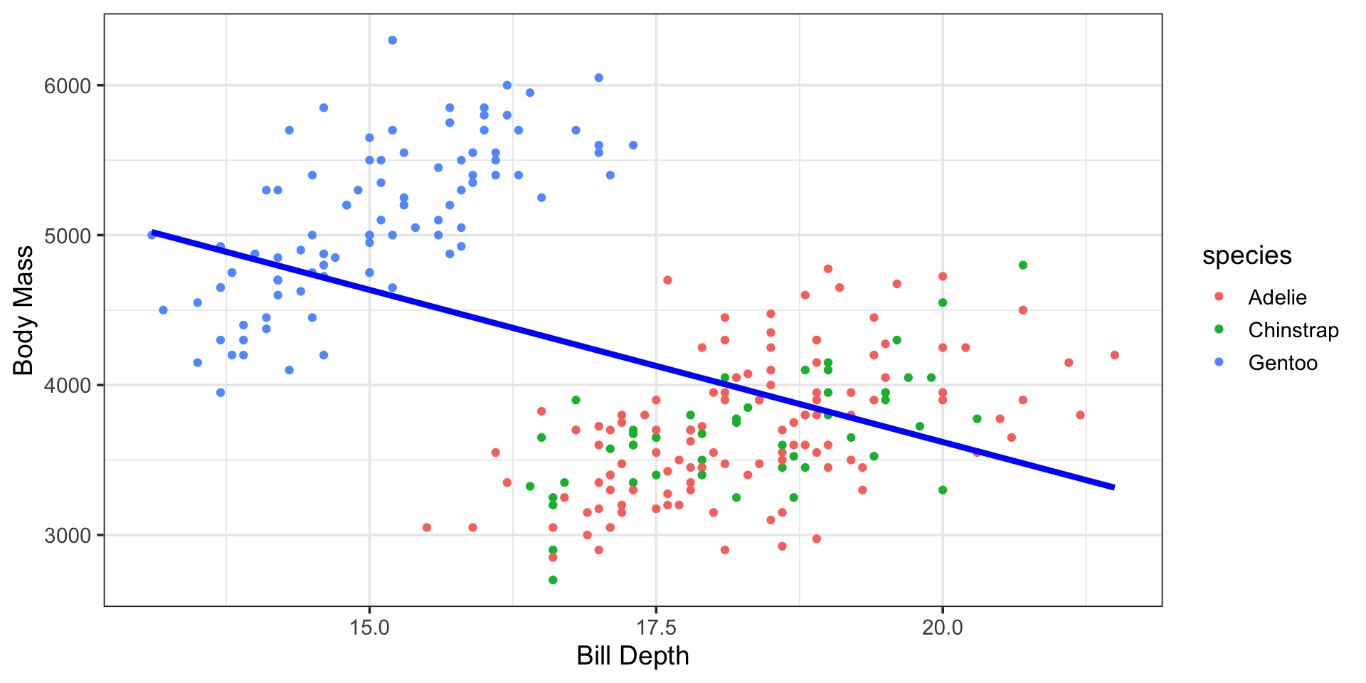
Let’s build a model that better corresponds to the plot we began this discussion with…

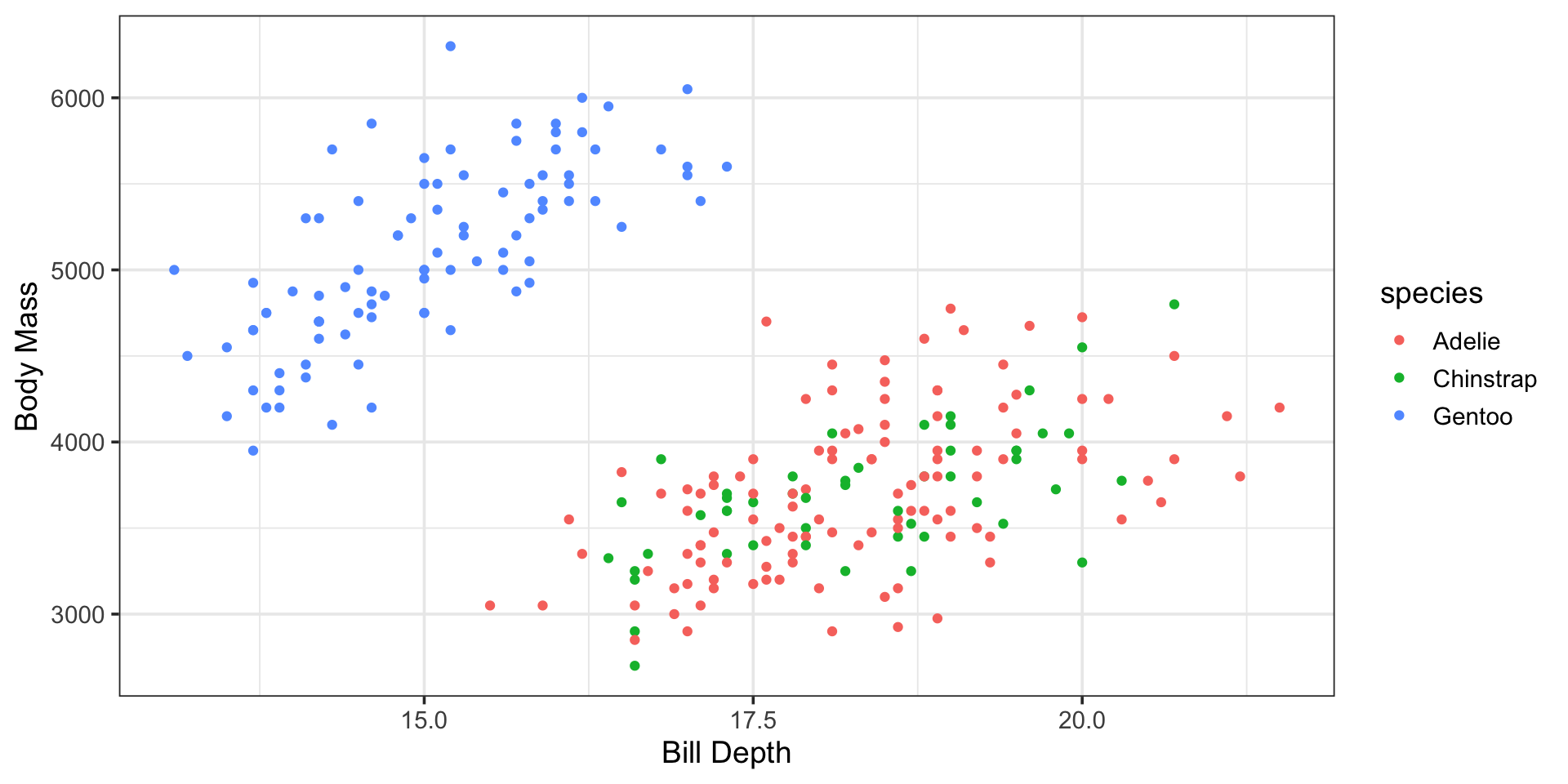
Can we accomodate both bill_depth_mm (a numerical variable) and species (a categorical variable) into a single model?

Bill Depth and Species as Predictors of Body Mass

Start with our model specification

lr_sbl_spec <- linear_reg() %>%
  set_engine("lm")

Now our recipe, with the feature engineering step included

lr_sbl_rec <- recipe(body_mass_g ~ bill_depth_mm + species, data = penguins_train) %>%
  step_dummy(species)

Next, we package both the model and recipe together into a workflow

lr_sbl_wf <- workflow() %>%
  add_model(lr_sbl_spec) %>%
  add_recipe(lr_sbl_rec)

And, finally, fit the workflow to the training data

lr_sbl_fit <- lr_sbl_wf %>%
  fit(penguins_train)

Important Note! Common concerns and remedies when including categorical predictors…

• step_unknown(cat_var_name) to fill in missing values with unknown
• step_novel(cat_var_name) to reassign new classes to a novel class
• step_other(cat_var_name) to combine rare classes into an other class

Models with Numerical and Categorical Predictors

\(\bigstar\) Let’s try it! \(\bigstar\)

1. Create an instance of a modeling workflow which uses at least one numerical predictor and at least one categorical predictor
2. Fit your workflow to your training data

Assessing Our New Model

Global Test for Model Utility:

lr_sbl_fit %>%
  glance()

r.squared	adj.r.squared	sigma	statistic	p.value	df	logLik	AIC	BIC	deviance	df.residual	nobs
0.7928019	0.7903352	375.7164	321.4091	0	3	-1879.014	3768.028	3785.754	35573029	252	256

Individual Term-Based Tests:

lr_sbl_fit %>%
  extract_fit_engine() %>%
  tidy(conf.int = TRUE)

term	estimate	std.error	statistic	p.value	conf.low	conf.high
(Intercept)	-912.90624	389.97673	-2.3409249	0.0200163	-1680.9351	-144.8773
bill_depth_mm	252.33546	21.22734	11.8872854	0.0000000	210.5299	294.1411
species_Chinstrap	-23.37012	63.73145	-0.3666969	0.7141529	-148.8843	102.1440
species_Gentoo	2220.99703	86.96707	25.5383665	0.0000000	2049.7221	2392.2719

Assessing Our New Model

Individual Term-Based Tests:

lr_sbl_fit %>%
  extract_fit_engine() %>%
  tidy(conf.int = TRUE)

term	estimate	std.error	statistic	p.value	conf.low	conf.high
(Intercept)	-912.90624	389.97673	-2.3409249	0.0200163	-1680.9351	-144.8773
bill_depth_mm	252.33546	21.22734	11.8872854	0.0000000	210.5299	294.1411
species_Chinstrap	-23.37012	63.73145	-0.3666969	0.7141529	-148.8843	102.1440
species_Gentoo	2220.99703	86.96707	25.5383665	0.0000000	2049.7221	2392.2719

Note: Controlling for differences in bill depth, all three species have statistically discernible average body masses

\[\begin{align} \mathbb{E}\left[\text{body mass}\right] \approx -912.91 ~+ &~252.34\cdot\left(\text{bill depth}\right) - 23.37\cdot\left(\text{speciesChinstrap}\right) +\\ &~2221.0\cdot\left(\text{speciesGentoo}\right)\end{align}\]

An Improvement Over the Species-Only Model?

Species-Only Model:

metric	value
r.squared	0.6766167
adj.r.squared	0.6740604
sigma	468.4530146
statistic	264.6767122
p.value	0.0000000
df	2.0000000
logLik	-1935.9949729
AIC	3879.9899458
BIC	3894.1706556
deviance	55520401.4016019
df.residual	253.0000000
nobs	256.0000000

Species and Bill Depth Model:

metric	value
r.squared	0.7928019
adj.r.squared	0.7903352
sigma	375.7164021
statistic	321.4091063
p.value	0.0000000
df	3.0000000
logLik	-1879.0141347
AIC	3768.0282694
BIC	3785.7541567
deviance	35573029.3286923
df.residual	252.0000000
nobs	256.0000000

Assessing and Comparing Models

\(\bigstar\) Let’s try it! \(\bigstar\)

1. Obtain and interpret your global and term-based model metrics
2. Compare your model’s training metrics to those of your previous models
3. Obtain performance metrics for this new model using the test data. How does this model perform on unknown test observations compared to your previous models?

Visualizing Model Coefficients

term	estimate	std.error	p.value	conf.low	conf.high
(Intercept)	-912.90624	389.97673	0.0200163	-1680.9351	-144.8773
bill_depth_mm	252.33546	21.22734	0.0000000	210.5299	294.1411
species_Chinstrap	-23.37012	63.73145	0.7141529	-148.8843	102.1440
species_Gentoo	2220.99703	86.96707	0.0000000	2049.7221	2392.2719

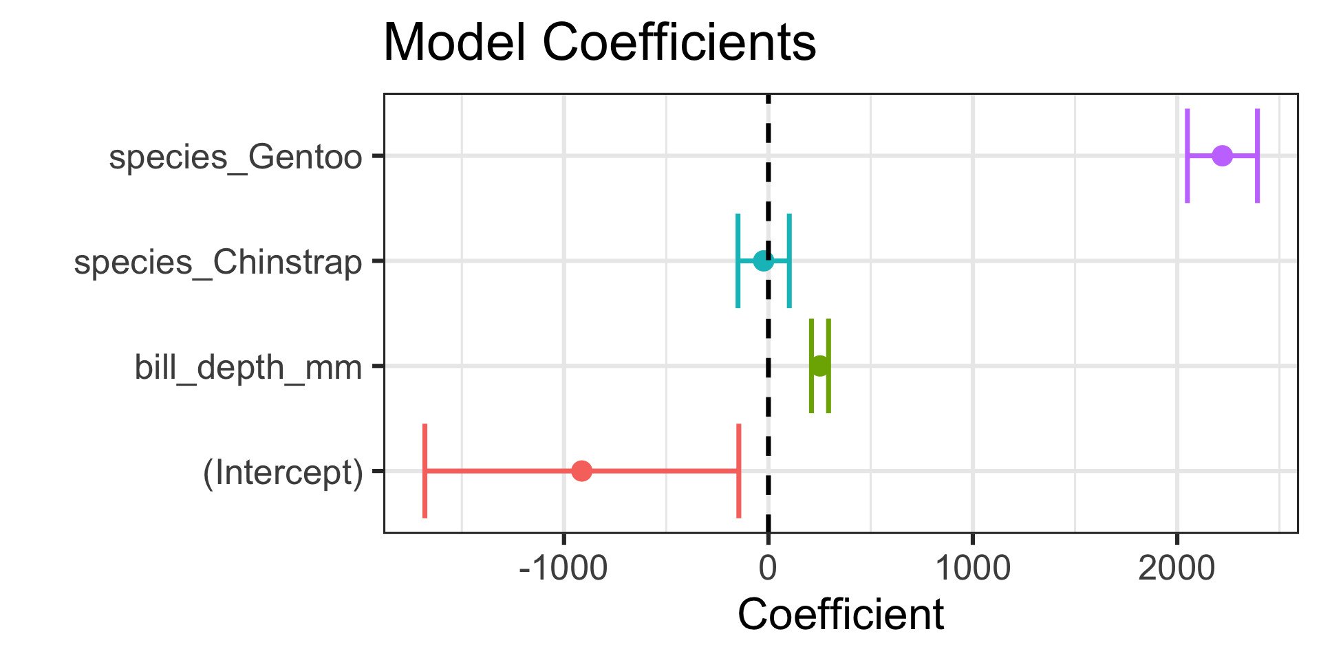
Visualizing Coefficients

\(\bigstar\) Let’s try it! \(\bigstar\)

1. Try to construct a plot which allows you to visualize your model coefficients and their plausible ranges.
2. What does the plot tell you about each model term?

Interpreting this Model

term	estimate	std.error	statistic	p.value
(Intercept)	-912.90624	389.97673	-2.3409249	0.0200163
bill_depth_mm	252.33546	21.22734	11.8872854	0.0000000
species_Chinstrap	-23.37012	63.73145	-0.3666969	0.7141529
species_Gentoo	2220.99703	86.96707	25.5383665	0.0000000

\[\begin{align} \mathbb{E}\left[\text{body mass}\right] \approx -912.91 ~+ &~252.34\cdot\left(\text{bill depth}\right) - 23.37\cdot\left(\text{speciesChinstrap}\right) +\\ &~2221.0\cdot\left(\text{speciesGentoo}\right)\end{align}\]

• (Intercept) Interpretation of this intercept is not meaningful because it would correspond to a penguin with a bill depth of 0mm.

• (Bill Depth) Controlling for differences in species, we expect a 1mm increase in bill depth to be associated with a 252.34g increase in body mass, on average.

• (Chinstrap) Given a Chinstrap and Adelie penguin with the same bill depth, we expect the Chinstrap to have a lower body mass by about 23.37g, on average.

• (Gentoo) Given a Gentoo and Adelie penguin with the same bill depth, we expect the Gentoo to have greater mass by about 2221.0g, on average.

  • Note: Some comparisons are misleading since Adelie bill depths rarely overlap with Gentoos’

Interpreting the Model

\(\bigstar\) Let’s try it! \(\bigstar\)

1. If you haven’t done so already, write down your estimated model form.
2. Interpret the intercept (if appropriate) and the estimated effect of each predictor on the response.

Making Predictions with this Model

new_data <- crossing(
  bill_depth_mm = seq(13.1, 21.5, length.out = 250),
  species = c("Adelie", "Chinstrap", "Gentoo")
)

new_data <- lr_sbl_fit %>%
  augment(new_data) %>%
  bind_cols(
    lr_sbl_fit %>%
      predict(new_data, type = "conf_int") %>%
      rename(
        .conf_lower = .pred_lower,
        .conf_upper = .pred_upper
      )
  ) %>%
  bind_cols(
    lr_sbl_fit %>%
      predict(new_data, type = "pred_int")
  )

Making Predictions with this Model

ggplot() + 
  geom_ribbon(data = new_data, 
              aes(x = bill_depth_mm, ymin = .pred_lower, ymax = .pred_upper),
              alpha = 0.25) +
  geom_ribbon(data = new_data,
              aes(x = bill_depth_mm, ymin = .conf_lower, ymax = .conf_upper),
              alpha = 0.5) +
  geom_line(data = new_data,
            aes(x = bill_depth_mm, y = .pred, color = species),
            lwd = 1.25) +
  geom_point(data = penguins_train,
             aes(x = bill_depth_mm, y = body_mass_g, color = species),
             alpha = 0.5) + 
  labs(
    x = "Bill Depth",
    y = "Body Mass"
  ) + 
  facet_wrap(~species, ncol = 3) + 
  theme(legend.position = "None")

Making Predictions with this Model

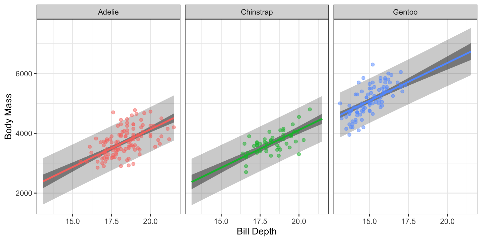
Note: Including the categorical predictor has resulted in our model taking the form of these separate, parallel lines.

Making and Visualizing Model Predictions

\(\bigstar\) Let’s try it! \(\bigstar\)

1. Create a counterfactual set of new observations using crossing()

2. Use your model to make predictions for those new observations

   • Include confidence intervals and prediction intervals as well

3. Create a graphical representation of your model’s predictions, including confidence- and prediction-bands

Additional Feature-Engineering Steps for Categorical Predictors

• If we expect to encounter missing values, we can use step_unknown() to create a level for unknown values or we can use step_impute_mode() to fill in missing levels with the most frequently observed level
• If we expect to encounter new levels, unknown to the model at training time, we can use step_novel()
• If we expect to have levels which are infrequently observed, we can group those levels together into an “other” level with step_other()

Summary

• We can include categorical predictors in a model to differentiate predictions across the levels of that variable

• Including categorical predictors in a model requires the use of an encoding scheme in order to convert levels to numerical values

  • Scoring assigns a distinct number to each category

    • Implement it by adding step_ordinalscore() as a feature engineering step in a recipe

  • Dummy encodings replace a categorical predictor with a collection of binary (0/1) variables indicating the levels of the categorical predictor

    • We can use the dummy variable technique by adding step_dummy() as a feature engineering step in a recipe

  • In the case of rare levels, we may want to also include step_other(), step_unknown(), or step_novel() as recipe steps as well – order of application matters!

• A linear regression model including a single categorical variable as the sole predictor is equivalent to ANOVA

• For a linear regression model with at least one numerical predictor, the result of the inclusion of a categorical variable in the model is a shift in intercept (a vertical shift) for each of the levels of the categorical predictor

Next Time…

Model-Building, Assessment, and Interpretation Workshop