Analysis of Residuals and Model Improvements

Dr. Gilbert

August 31, 2024

Motivation

\[\mathbb{E}\left[y\right] = \beta_0 + \beta_1 x_1 + \beta_2 x_2 + \beta_3 x_3\]

Motivation

\[\mathbb{E}\left[y\right] = \beta_0 + \beta_1 x_1 + \beta_2 x_2 + \beta_3 x_3\]

Motivation

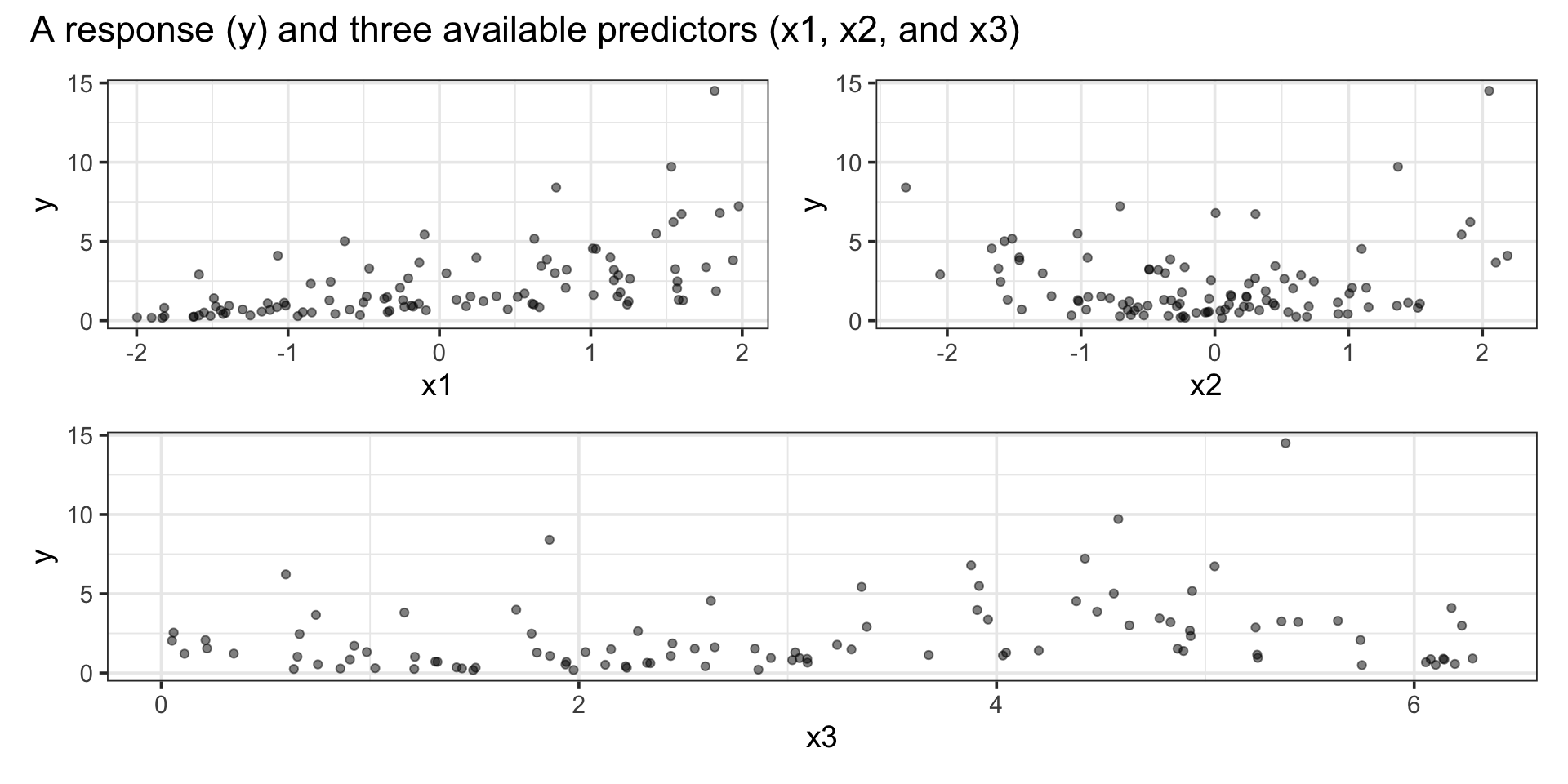
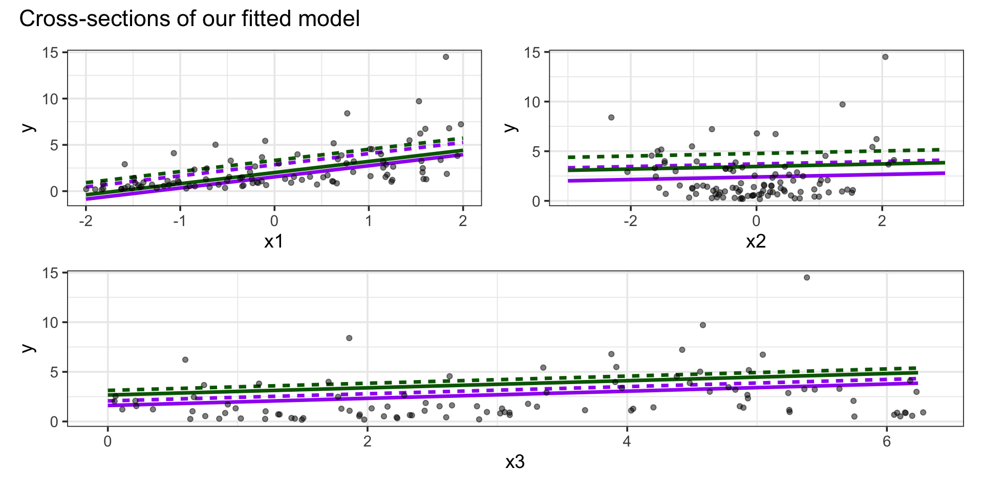
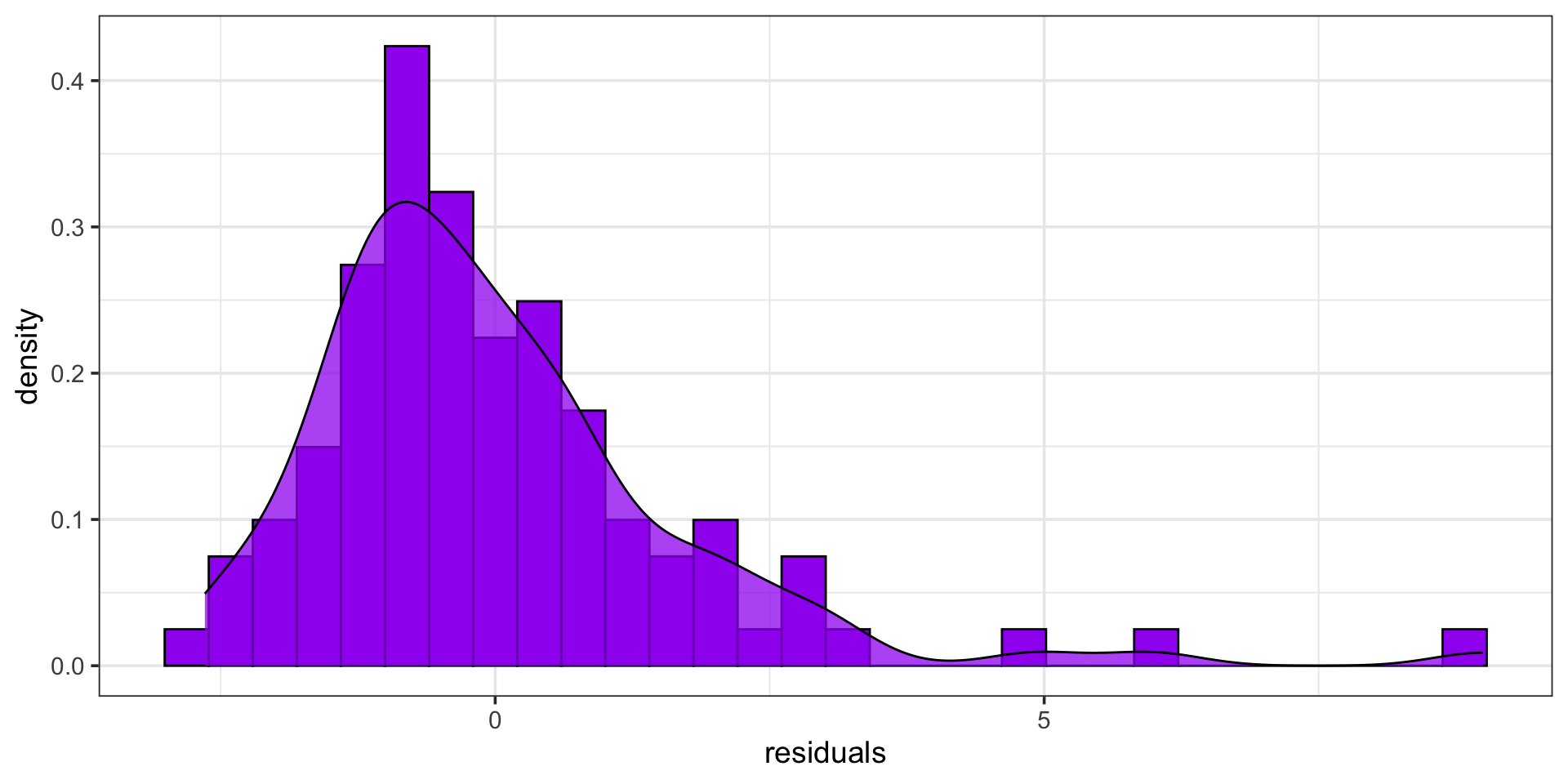
Now that we have a fitted model, let’s check out the residuals

Motivation

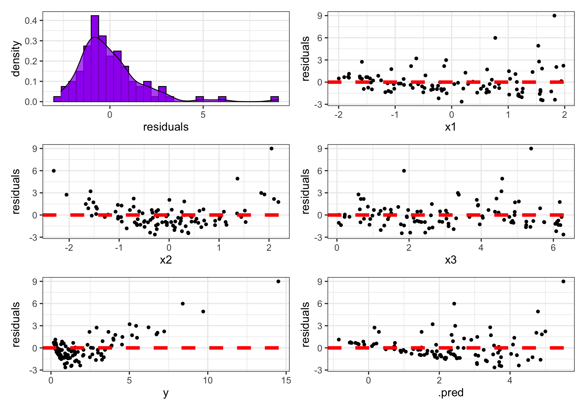
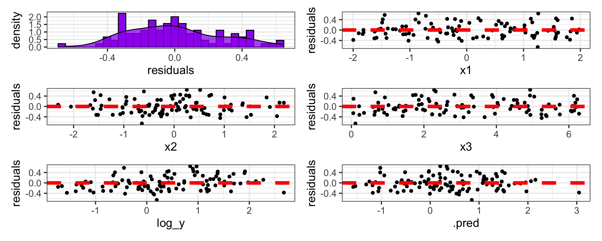
The residual plots indicate some badness

• Residuals are not normally distributed

• Residuals don’t seem to be random

  • Residuals show patterns with respect to some predictors and the response

• Variance of residuals is not constant

The Highlights

• Types of residual plots

  • Plotting the distribution of residuals
  • Residuals versus the response
  • Residuals versus fitted values (model predictions)
  • Residuals versus predictors

• Reactions to problematic residual plots

  • Transformations of the response variable
  • Transformations of the predictor(s)
  • (\(\bigstar\) Later In Our Course \(\bigstar\)) Choosing a different model class altogether

A Note on Structure: This notebook will alternate between examining a particular type of residual plot and then identifying and executing a potential remedy for problematic results involving residuals.

Types of Residual Plot: Distribution of Residuals

Purpose: A plot of the distribution of residuals tells us whether our model results in prediction errors (residuals) that are normally distributed.

Why Care? Normal distribution of residuals is the assumption that allows us to build meaningful confidence- and prediction-intervals for the responses of new observations.

Responding to Non-Normal Residuals

Remedies for Non-Normal Residuals: Residuals being non-normally distributed is usually due to skew in the distribution of the response variable. We can model transformations of the response (ie. predicting \(\ln\left(y\right)\), \(\exp\left(y\right)\), \(\sqrt{y}\), etc.) instead of directly modeling \(y\).

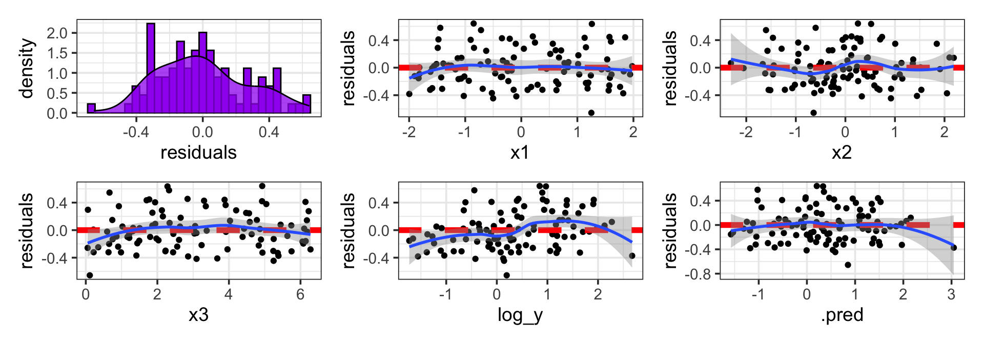
In the case of skewed residuals, like we see here, a reasonable approach is to model \(\ln\left(y\right)\) rather than modeling \(y\) directly.

Let’s make that change to our modeling strategy and revising the resulting residual plots.

Updating Our Model (Transformed Response)

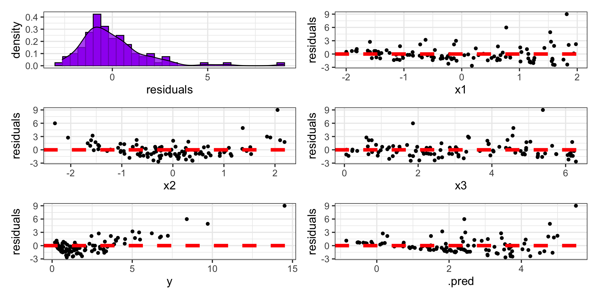
As a reminder, in the residual plots below, we’ve chosen to model the logarithm of \(y\) instead of modeling \(y\) directly.

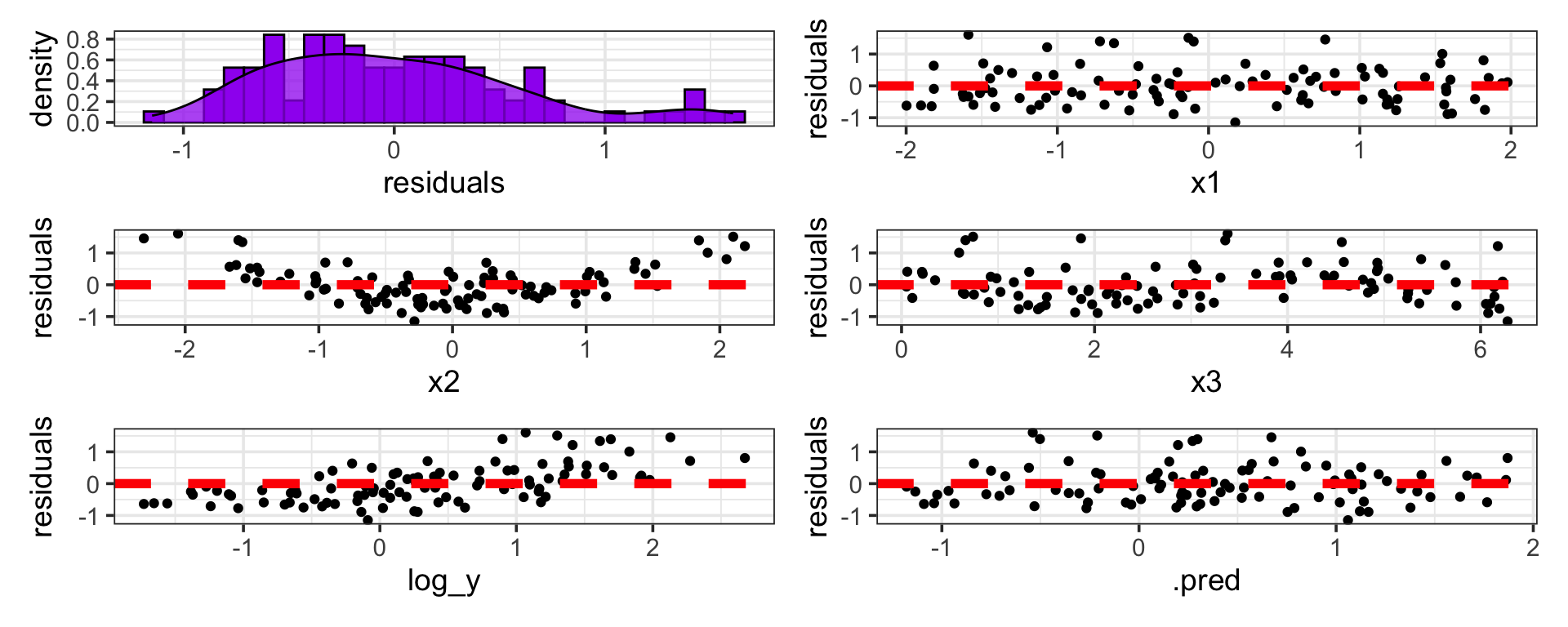
Certainly, this distribution of residuals is not perfectly normal, but it’s better!

We seem to have fixed the issue of non-constant variance with respect to model predictions (fitted values)

…and improved, but not eliminated, the issue of the association between residuals and the response.

Types of Residual Plot: Residuals versus Predictors

Purpose: A plot exploring potential associations between residuals and our utilized predictors tells us whether associations between the predictor and response are non-linear.

Why Care: We can adjust how we utilize our predictors in-model to obtain better predictive performance and descriptive properties.

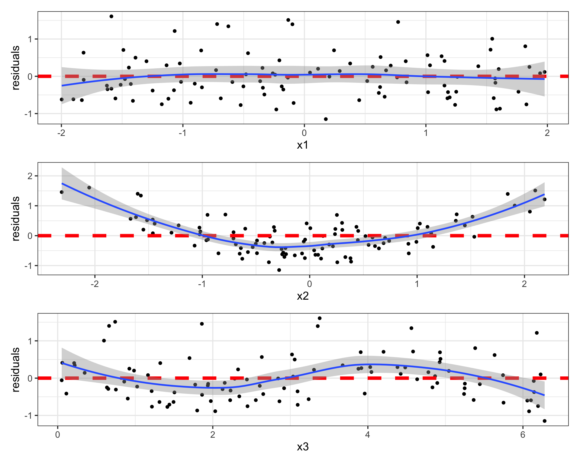
• There seems to be no association between the residuals and x1
• There is curvature in the association between the residuals and x2
• And curvature of a different type between the residuals and x3

Responding to Associations Between Residuals and Predictors

Remedies for Associations Between Residuals and Predictors: We can improve model fit (and perhaps explanatory value) by employing transforms of predictors.

• No transformation of x1 is necessary
• The curved association between the residuals and x2 indicates that perhaps a quadratic association between x2 and \(\ln\left(y\right)\) exists.
• The curved association between the residuals and x3 indicates that perhaps a cubic or sinusoidal association between x3 and \(\ln\left(y\right)\) exists.

Again, we’ll make these model updates (I’ll show you how in the coming days) and revisit our residual plots for the updated model.

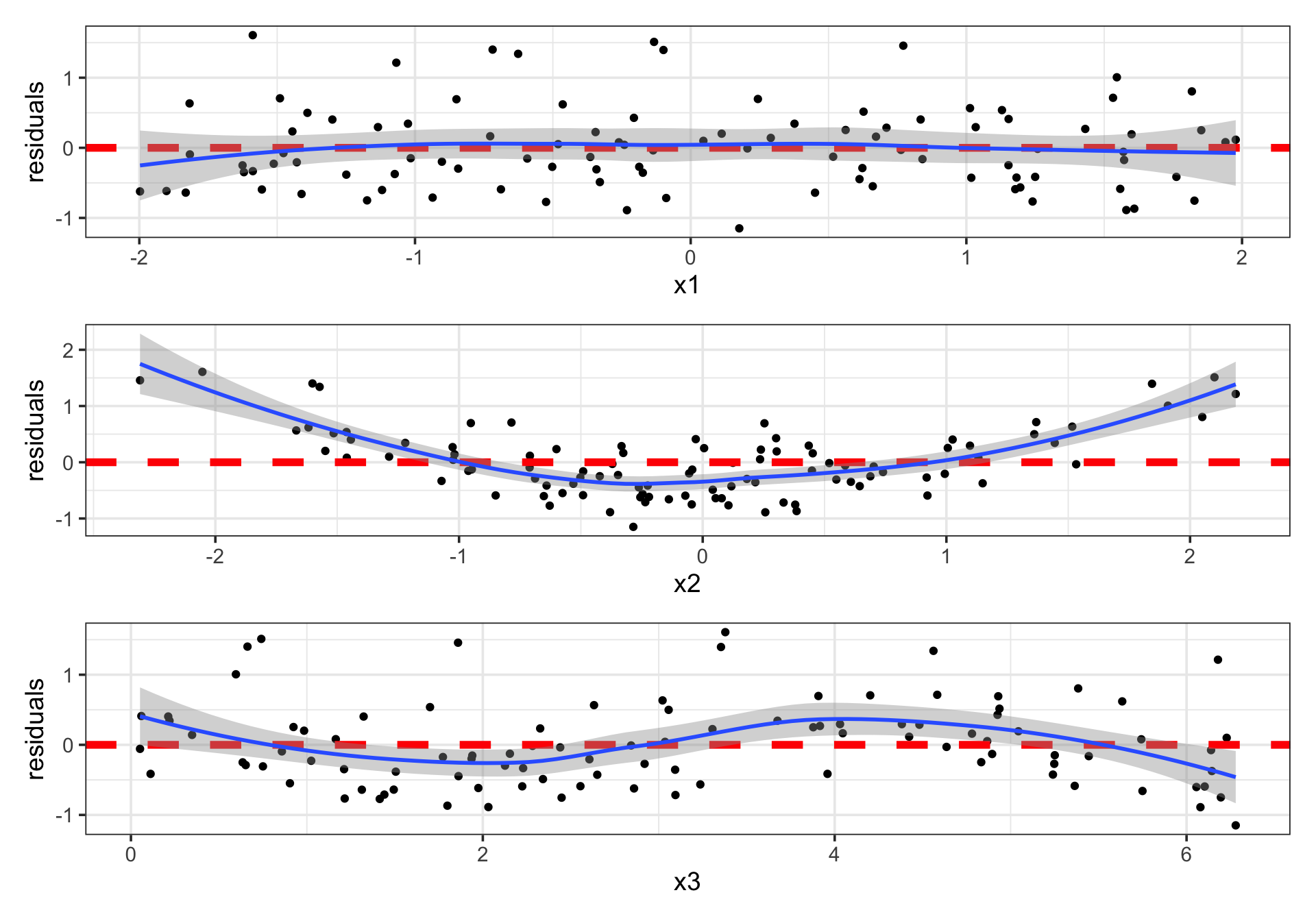
Updating Our Model (Transformed Predictors)

As a reminder, in the residual plots below, we’ve chosen to model the logarithm of \(y\) instead of modeling \(y\) directly. We’ve also included a quadratic term corresponding to the x2 predictor and we’re using sin(x3) in the model instead of x3 directly.

Again, nothing is exactly perfect in these residual plots, but…

Updating Our Model (Transformed Predictors)

• The residuals are approximately normally distributed (with a spike near -0.3, which we should investigate)

• The variance in residuals seems constant with respect to predictors, response, and predicted values

  • We can have more trust in our confidence and prediction intervals

• There are no remaining associations between the residuals and the predictors

  • We are confident that we’ve squeezed out predictive value

Summary

• An analysis of residuals provides insight into model deficiencies

• If residuals are not normally distributed, with a constant standard deviation, then we cannot trust our confidence- or prediction-intervals

  • In the case of non-normally distributed residuals or non-constant variance, we can try transformations of the response variable
  • This includes modeling the logarithm of the response, taking the exponential of the response, the square root of the response, etc.

• If associations exist between the residuals and available predictors, then we’ve “left predictive power on the table”

  • We can explore transformations of the predictors in order to gain predictive accuracy and explanatory value
  • This can include raising predictors to a power, combining predictors together, applying trigonometric functions to predictors – anything you can justify!

• If associations exist between the residuals and either the response or the model’s predicted values, then this means your model makes different errors depending on either the magnitude of the response or the magnitude of the predictions (ie. big response, big error / small response, small error)

  • In this case confidence- and prediction-intervals cannot be trusted
  • Exploring transformations of either the response or predictors can help here

Next Time…

Categorical Predictors and Interpretations