Topic 15: Hypothesis Tests and Confidence Intervals for Numerical Data (Spreadsheets)

About

This activity introduces techniques for inference on a single population mean and for comparing two population means. The \(t\)-distributions are introduced, historical context is provided, and we work through two applications using federal sentencing data on drug-related convictions from the Southern District of New York State.

{
  const btn = html`<button style="
    background: #436b95;
    color: white;
    border: none;
    padding: 8px 16px;
    border-radius: 4px;
    cursor: pointer;
    font-size: 0.9em;
  ">🔄 Reset My Responses</button>`;

  btn.onclick = () => {
    if (confirm('Reset all responses for this activity? This cannot be undone.')) {
      Object.keys(localStorage)
        .filter(k => k.endsWith('_selected_t15e') || k.endsWith('_correct_t15e') || k.endsWith('_result_t15e'))
        .forEach(k => localStorage.removeItem(k));
      location.reload();
    }
  };

  return btn;
}

Note. The button above resets multiple choice and checkbox questions. Currently, resetting answer entry cells must be done manually via hitting the Start Over button on each individual interactive cell.

Using a Spreadsheet Program

Through the beginning of this activity, you’ll be asked to use empty cells on a blank excel sheet for calculations. After this initial section, you’ll work with actual criminal sentencing data from the Southern District of New York State. Use the links below to obtain a copy of the spreadsheet containing the relevant data.

If you are a Google Sheets user, click here to create a copy of the spreadsheet for this activity
If you are an Excel user, click here to download a copy of the spreadsheet for this activity

Hypothesis Testing and Confidence Intervals for Numerical Data

In this activity, we continue our exploration of statistical inference. Through the past few activities you’ve become more comfortable with hypothesis testing and confidence intervals for categorical variables. Here we extend those frameworks to numerical variables. We’ll first be formally introduced to the family of \(t\)-distributions, and then work through a pair of applications to real criminal sentencing data.

As a reminder, the Standard Error Decision Tree, General Strategy for Conducting Hypothesis Tests, and General Strategy for Constructing Confidence Intervals are all available for reference. The walkthrough video for the decision tree is below, in case you’d like a refresher.

While watching the walkthrough video you probably noticed that the side of the decision tree corresponding to numerical data (inference for the mean, \(\mu\)) is more complex than the side for proportions. Much of this stems from the fact that using a sample standard deviation (\(s\)) as an approximation for the population standard deviation (\(\sigma\)) adds uncertainty to our estimate of the sampling distribution. To account for this added uncertainty, we utilize a class of penalized normal distributions called the \(t\)-distributions. Watch at least one of the introductory videos below.

A Detailed Introduction:

A Shorter Introduction:

What Does the \(t\)-Distribution Look Like?

The videos above have helped us identify scenarios where we should utilize a \(t\)-distribution instead of the standard normal (\(z\)) distribution. There is a simple rule to follow that will help you decide which distribution to use: any time we use a sample standard deviation as a proxy for the population standard deviation in our estimate for the standard error, we should use a \(t\)-distribution.

The plot below shows the standard normal distribution in black, a \(t\)-distribution with 3 degrees of freedom in red, and a \(t\)-distribution with 12 degrees of freedom in blue.

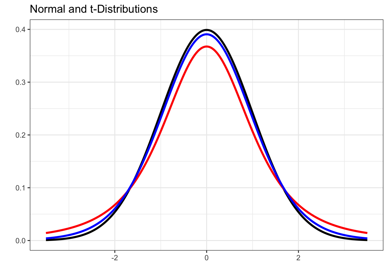
Notice that all three distributions are bell-shaped, but the \(t\)-distributions have fatter tails than the normal distribution. This means that the \(t\)-distributions have more area/probability in their tails than the standard normal distribution. Also notice that the \(t\)-distribution with 12 degrees of freedom is more similar to the standard normal distribution than the one with 3 degrees of freedom. As degrees of freedom increase, the \(t\)-distribution approaches (becomes more like) the normal distribution.

Using the \(t\)-Distributions

When we introduced the normal distribution, we identified two helper functions that you could use in your spreadsheet formulas: NORM.DIST() to find probabilities (areas to the left of a boundary value) and NORM.INV() to find percentile cutoffs. We have analogous functions for the \(t\)-distribution:

=T.DIST(q, df, TRUE) — finds the probability of a randomly chosen observation falling to the left of the boundary value q in a \(t\)-distribution with df degrees of freedom.
=T.INV(p, df) — finds the cutoff value for which the area to the left of that cutoff in a \(t\)-distribution with df degrees of freedom is p.

Note that unlike NORM.DIST() and NORM.INV(), these functions have no mean or standard deviation arguments — we always work with standardized variables (via the test statistic formula) when using the \(t\)-distributions.

Let’s practice. Don’t forget to draw pictures — you are much more likely to make mistakes if you skip this step. Use the BlankSheet tab of the spreadsheet you copied at the beginning of this activity for your calculations.

Question 1: Find \(\mathbb{P}\left[t <\right.\) \(\left.\right]\) in a \(t\)-distribution with degrees of freedom.

In your spreadsheet, compute this probability and enter your result below.


pt(boundary1, df = df1)

Question 2: Find \(\mathbb{P}\left[t >\right.\) \(\left.\right]\) in a \(t\)-distribution with degrees of freedom.

In your spreadsheet, compute this probability and enter your result below.


1 - pt(boundary2, df = df2)

Question 3: Find the cutoff value in a \(t\)-distribution with degrees of freedom for which the area to the left of the cutoff is .

In your spreadsheet, compute this cutoff and enter your result below.


qt(area3, df = df3)

Question 4: Find the critical value associated with a % confidence interval using a \(t\)-distribution with degrees of freedom.

In your spreadsheet, compute this critical value and enter your result below.


qt(1 - (1 - clevel4/100)/2, df = df4)

Summary: Working with the \(t\)-Distributions

We’ve now practiced with two spreadsheet new functions for working with \(t\)-distributions:

=T.DIST(q, df, TRUE) — returns the area to the left of the boundary value q in a \(t\)-distribution with df degrees of freedom. This is the \(t\)-distribution analog of =NORM.DIST(q, 0, 1, TRUE).
=T.INV(p, df) — returns the boundary value for which the area to the left is p in a \(t\)-distribution with df degrees of freedom. This is the \(t\)-distribution analog of =NORM.INV(p, 0, 1).

As with the normal distribution, you will need to think carefully about how to use these functions to obtain the quantities (areas/probabilities or boundary values) that you are looking for. Drawing a picture will help you.

Applications to Criminal Sentencing

We’ll work with a dataset on Federal Sentencing from the Southern District of New York State. The full dataset is available to you on the SDNYfull tab of the spreadsheet you copied at the beginning of this activity, and the records filtered to only include sentences from drug-related convictions is available on the SDNYdrug tab.

Open you spreadsheet and switch to the SDNYdrug tab. You’ll complete the work for the next scenarios on that tab.

Spreadsheet Tips to Remember

You’ll benefit by recalling and refreshing on the following items. Check back in on the Topic 2: Introduction to Spreadsheets and Topic 3: Descriptive Statistics activities for more details.

Working with ranges of cells is done via top_left_cell:bottom_right_cell. That is, C2:F23 selects all the cells in the rectangular grid from cell C2 (third column, second row) to cell F23 (sixth colum, twenty-third row). Similarly, C2:C500 selects all the cells in column C between row 2 and row 500.
Spreadsheet software has built-in functions like AVERAGE(), STDEV(), COUNT(), and more that allow you to quickly run calculations over a range.
Creating grouped summaries can be done via Pivot Tables. You create a pivot table by clicking on a cell inside of your data range, navigating to Insert, and then choosing Pivot Table.

There will be robust hint sequences to help you along the way when you get stuck.

Task 1: Confidence Interval for Average Sentence Length

Construct a 95% confidence interval for the average sentence length for a drug-related conviction in the Southern District of New York State.

Check Your Understanding: Sentencing CI, Part I

To answer the question as asked, we should:

mutable ok_response = (response, n) => { return html`Loading...` };
viewof q1 = Inputs.radio(
  new Map([
    ["Compute a probability.", 1],
    ["Construct a confidence interval.", 2],
    ["Conduct a hypothesis test.", 3],
    ["Calculate a required sample size.", 4]
  ]),
  {value: JSON.parse(localStorage.getItem("q1_selected_t15e") ?? "null")}
);

{
  localStorage.setItem("q1_selected_t15e", JSON.stringify(q1));
  localStorage.setItem("q1_correct_t15e", "2");
  localStorage.setItem("q1_result_t15e", q1 === null ? "unattempted" : (q1 == 2 ? "correct" : "incorrect"));
}

ok_response(q1, "2");

Use an empty cell on the SDNYdrug tab of your spreadsheet to calculate the average sentence length for drug-related convictions in the Southern District of New York State. Enter your result in the code cell below.

mean(SDNYdrug$SentenceMonths)

Check Your Understanding: Sentencing CI, Part II

The standard error formula is:

viewof q2 = Inputs.radio(
  new Map([
    ["SE = sqrt(p(1-p)/n)", 1],
    ["SE = σ/sqrt(n)", 2],
    ["SE = s/sqrt(n)", 3],
    ["SE = sqrt(p1(1-p1)/n1 + p2(1-p2)/n2)", 4],
    ["SE = sqrt(s1²/n1 + s2²/n2)", 5]
  ]),
  {value: JSON.parse(localStorage.getItem("q2_selected_t15e") ?? "null")}
);

{
  localStorage.setItem("q2_selected_t15e", JSON.stringify(q2));
  localStorage.setItem("q2_correct_t15e", "3");
  localStorage.setItem("q2_result_t15e", q2 === null ? "unattempted" : (q2 == 3 ? "correct" : "incorrect"));
}

ok_response(q2, "3");

Hint 1

Open the Standard Error Decision Tree and start from the top of the tree.

Hint 2

Are we conducting inference on a mean (\(\mu\)) or a proportion (\(p\))?

Hint 3

The question “How long was the sentence associated with this conviction?” is answered with a number of months. This is numerical data that is best summarized by a mean. We’re on the right side of the tree.

Hint 4

How many groups/populations are we comparing? Do we know the population standard deviation, \(\sigma\)?

Hint 5

We have just a single population here – all of the individual sentences belong to one group. We don’t know the population standard deviation in sentence lengths.

Note that we can calculate the standard deviation in sentence lengths, but that will only the the standard deviation for the sentences in our sample (\(s\)).

What is the standard error (\(S_E\)) from the box you landed in?

Using your spreadsheet, calculate the standard error for the average sentence length.


sd(SDNYdrug$SentenceMonths) / sqrt(nrow(SDNYdrug))

Check Your Understanding: Sentencing CI, Part III

The distribution to be used is:

viewof q3 = Inputs.radio(
  new Map([
    ["Normal.", 1],
    ["t-distribution with df = n - 1.", 2],
    ["t-distribution with df = min(n1-1, n2-1).", 3],
    ["t-distribution with df = n_diff - 1.", 4],
    ["We should not use either distribution.", 5]
  ]),
  {value: JSON.parse(localStorage.getItem("q3_selected_t15e") ?? "null")}
);

{
  localStorage.setItem("q3_selected_t15e", JSON.stringify(q3));
  localStorage.setItem("q3_correct_t15e", "2");
  localStorage.setItem("q3_result_t15e", q3 === null ? "unattempted" : (q3 == 2 ? "correct" : "incorrect"));
}

ok_response(q3, "2");

Hint 1

The *Standard Error Decision Tree tells you which distribution to use.

Hint 2

Check the box you landed in when finding the standard error (\(S_E\)) formula.

Hint 3

If that box is not a specialty box (ANOVA or \(\chi^2\)) and it contains information about degrees of freedom (\(df\)), then you’re using a \(t\)-distribution with that number of degrees of freedom. Otherwise, you’re using the normal distribution.

Check Your Understanding: Sentencing CI, Part IV

The desired level of confidence is:

viewof q4 = Inputs.radio(
  new Map([
    ["90%", 1],
    ["0.95%", 2],
    ["95%", 3],
    ["98%", 4],
    ["99%", 5]
  ]),
  {value: JSON.parse(localStorage.getItem("q4_selected_t15e") ?? "null")}
);

{
  localStorage.setItem("q4_selected_t15e", JSON.stringify(q4));
  localStorage.setItem("q4_correct_t15e", "3");
  localStorage.setItem("q4_result_t15e", q4 === null ? "unattempted" : (q4 == 3 ? "correct" : "incorrect"));
}

ok_response(q4, "3");

Now use your spreadsheet to compute the critical value for the confidence interval and enter your result below.


qt(0.975, df = nrow(SDNYdrug) - 1)

A Note on the Critical Value

With so many observations, the correct critical value differs very little from 1.96 (the value obtained from the normal distribution). Remember that the critical values on the Standard Error Decision Tree are for the normal distribution only. Any time we use a sample standard deviation as a stand-in for the population standard deviation, we should use T.INV() — this will make a larger difference when sample sizes are smaller.

Now use your spreadsheet to compute the lower bound of the 95% confidence interval and enter your result below.


mean(SDNYdrug$SentenceMonths) - 
  qt(0.975, df = nrow(SDNYdrug) - 1) * 
  (sd(SDNYdrug$SentenceMonths) / sqrt(nrow(SDNYdrug)))

Now compute the upper bound and enter your result below.


mean(SDNYdrug$SentenceMonths) + 
  qt(0.975, df = nrow(SDNYdrug) - 1) * 
  (sd(SDNYdrug$SentenceMonths) / sqrt(nrow(SDNYdrug)))

Check Your Understanding: Sentencing CI, Part V

Which of the following is the correct interpretation of this confidence interval?

viewof q5 = Inputs.radio(
  new Map([
    ["95% of sentence lengths for drug-related charges in the Southern District of New York State will fall between the lower and upper bounds.", 1],
    ["We are 95% confident that the average sentence length for drug-related crimes in this sample falls between the lower and upper bounds.", 2],
    ["There is a 95% chance a criminal charged with a drug-related offense will receive a sentence between the lower and upper bounds.", 3],
    ["We are 95% confident that the true average sentence length for drug-related offenders in the Southern District of New York State is between the lower and upper bounds calculated.", 4]
  ]),
  {value: JSON.parse(localStorage.getItem("q5_selected_t15e") ?? "null")}
);

{
  localStorage.setItem("q5_selected_t15e", JSON.stringify(q5));
  localStorage.setItem("q5_correct_t15e", "4");
  localStorage.setItem("q5_result_t15e", q5 === null ? "unattempted" : (q5 == 4 ? "correct" : "incorrect"));
}

ok_response(q5, "4");

Check Your Understanding: Sentencing CI, Part VI

Does this sample provide evidence to suggest that the average sentence length for drug-related charges in the Southern District of New York State exceeds three years (36 months)?

viewof q6 = Inputs.radio(
  new Map([
    ["No. The confidence interval shows that an average sentence below 36 months is plausible.", 1],
    ["Yes. The confidence interval for the average sentence length includes only values exceeding 36 months.", 2],
    ["No. Some sentence lengths are below 36 months while others exceed 36 months.", 3],
    ["It is impossible to say, since a different sample would result in a different confidence interval.", 4]
  ]),
  {value: JSON.parse(localStorage.getItem("q6_selected_t15e") ?? "null")}
);

{
  localStorage.setItem("q6_selected_t15e", JSON.stringify(q6));
  localStorage.setItem("q6_correct_t15e", "2");
  localStorage.setItem("q6_result_t15e", q6 === null ? "unattempted" : (q6 == 2 ? "correct" : "incorrect"));
}

ok_response(q6, "2");

Task 2: Hypothesis Test for Difference in Sentence Lengths

Conduct a hypothesis test at the \(\alpha = 0.10\) level of significance to determine whether the sample data provides significant evidence that the average sentence length for white offenders and the average sentence length for non-white offenders differs for drug-related cases in the Southern District of New York State.

Check Your Understanding: Sentencing HT, Part I

To answer the question as asked, we should:

viewof q7 = Inputs.radio(
  new Map([
    ["Compute a probability.", 1],
    ["Construct a confidence interval.", 2],
    ["Conduct a hypothesis test.", 3],
    ["Calculate a required sample size.", 4]
  ]),
  {value: JSON.parse(localStorage.getItem("q7_selected_t15e") ?? "null")}
);

{
  localStorage.setItem("q7_selected_t15e", JSON.stringify(q7));
  localStorage.setItem("q7_correct_t15e", "3");
  localStorage.setItem("q7_result_t15e", q7 === null ? "unattempted" : (q7 == 3 ? "correct" : "incorrect"));
}

ok_response(q7, "3");

Check Your Understanding: Sentencing HT, Part II

What is the level of significance associated with this test?

viewof q8 = Inputs.radio(
  new Map([
    ["α = 0.01", 1],
    ["α = 0.05", 2],
    ["α = 0.10", 3],
    ["The p-value.", 4]
  ]),
  {value: JSON.parse(localStorage.getItem("q8_selected_t15e") ?? "null")}
);

{
  localStorage.setItem("q8_selected_t15e", JSON.stringify(q8));
  localStorage.setItem("q8_correct_t15e", "3");
  localStorage.setItem("q8_result_t15e", q8 === null ? "unattempted" : (q8 == 3 ? "correct" : "incorrect"));
}

ok_response(q8, "3");

Check Your Understanding: Sentencing HT, Part III

Does this hypothesis test involve testing a statement about a mean (\(\mu\)), a proportion (\(p\)), or something else?

viewof q9 = Inputs.radio(
  new Map([
    ["One or more means.", 1],
    ["One or more proportions.", 2],
    ["Something else altogether.", 3]
  ]),
  {value: JSON.parse(localStorage.getItem("q9_selected_t15e") ?? "null")}
);

{
  localStorage.setItem("q9_selected_t15e", JSON.stringify(q9));
  localStorage.setItem("q9_correct_t15e", "1");
  localStorage.setItem("q9_result_t15e", q9 === null ? "unattempted" : (q9 == 1 ? "correct" : "incorrect"));
}

ok_response(q9, "1");

Check Your Understanding: Sentencing HT, Part IV

How many groups are being compared in this test?

viewof q10 = Inputs.radio(
  new Map([
    ["The test involves only a single group.", 1],
    ["The test compares two groups.", 2],
    ["The test compares more than two groups.", 3]
  ]),
  {value: JSON.parse(localStorage.getItem("q10_selected_t15e") ?? "null")}
);

{
  localStorage.setItem("q10_selected_t15e", JSON.stringify(q10));
  localStorage.setItem("q10_correct_t15e", "2");
  localStorage.setItem("q10_result_t15e", q10 === null ? "unattempted" : (q10 == 2 ? "correct" : "incorrect"));
}

ok_response(q10, "2");

Check Your Understanding: Sentencing HT, Part V

Which of the following are the hypotheses associated with this test?

viewof q11 = Inputs.radio(
  new Map([
    ["H₀: μ_white − μ_nonwhite = 0; Hₐ: μ_white − μ_nonwhite ≠ 0", 1],
    ["H₀: μ_white − μ_nonwhite = 0; Hₐ: μ_white − μ_nonwhite > 0", 2],
    ["H₀: μ_white − μ_nonwhite = 0; Hₐ: μ_white − μ_nonwhite < 0", 3],
    ["H₀: μ_white ≠ μ_nonwhite; Hₐ: μ_white = μ_nonwhite", 4]
  ]),
  {value: JSON.parse(localStorage.getItem("q11_selected_t15e") ?? "null")}
);

{
  localStorage.setItem("q11_selected_t15e", JSON.stringify(q11));
  localStorage.setItem("q11_correct_t15e", "1");
  localStorage.setItem("q11_result_t15e", q11 === null ? "unattempted" : (q11 == 1 ? "correct" : "incorrect"));
}

ok_response(q11, "1");

Hint 1

The null hypothesis (\(H_0\)) is a skeptical claim – “there’s nothing to see here”, while the alternative hypothesis (\(H_a\)) is the claim to be tested.

Hint 2

The claim we’re investigating asks whether or not there is a difference in the average sentence lengths.

Check Your Understanding: Sentencing HT VI

Do we know the population standard deviations (\(\sigma\)) for sentence lengths in each group?

viewof q12 = Inputs.radio(
  new Map([
    ["Yes, we can compute the population standard deviation from the data using STDEV().", 1],
    ["Yes, we are provided the population standard deviation.", 2],
    ["No — STDEV() would help us find the sample standard deviation, not the population standard deviation.", 3]
  ]),
  {value: JSON.parse(localStorage.getItem("q12_selected_t15e") ?? "null")}
);

{
  localStorage.setItem("q12_selected_t15e", JSON.stringify(q12));
  localStorage.setItem("q12_correct_t15e", "3");
  localStorage.setItem("q12_result_t15e", q12 === null ? "unattempted" : (q12 == 3 ? "correct" : "incorrect"));
}

ok_response(q12, "3");

Check Your Understanding: Sentencing HT, Part VII

Are the observations in the two groups (sentences handed to white offenders and sentences handed to non-white offenders) paired?

viewof q13 = Inputs.radio(
  new Map([
    ["No. There is no reason to suggest that sentences are paired.", 1],
    ["Yes. Every sentence handed to a white offender can be naturally paired with a sentence handed to a non-white offender.", 2]
  ]),
  {value: JSON.parse(localStorage.getItem("q13_selected_t15e") ?? "null")}
);

{
  localStorage.setItem("q13_selected_t15e", JSON.stringify(q13));
  localStorage.setItem("q13_correct_t15e", "1");
  localStorage.setItem("q13_result_t15e", q13 === null ? "unattempted" : (q13 == 1 ? "correct" : "incorrect"));
}

ok_response(q13, "1");

Check Your Understanding: Sentencing HT, Part VIII

Which standard error formula should be used?

viewof q14 = Inputs.radio(
  new Map([
    ["SE = s/sqrt(n)", 1],
    ["SE = sqrt(s1²/n1 + s2²/n2)", 2],
    ["SE = sqrt(σ1²/n1 + σ2²/n2)", 3],
    ["SE = sqrt(p(1-p)/n)", 4]
  ]),
  {value: JSON.parse(localStorage.getItem("q14_selected_t15e") ?? "null")}
);

{
  localStorage.setItem("q14_selected_t15e", JSON.stringify(q14));
  localStorage.setItem("q14_correct_t15e", "2");
  localStorage.setItem("q14_result_t15e", q14 === null ? "unattempted" : (q14 == 2 ? "correct" : "incorrect"));
}

ok_response(q14, "2");

Hint 1

Walk through the standard error decision tree using the answers to the questions above.

Check Your Understanding: Sentencing HT IX

Which distribution does the test statistic follow?

viewof q15 = Inputs.radio(
  new Map([
    ["The normal distribution.", 1],
    ["The t-distribution with df = n - 1.", 2],
    ["The t-distribution with df = min(n1 - 1, n2 - 1).", 3],
    ["The t-distribution with df = n_diff - 1.", 4]
  ]),
  {value: JSON.parse(localStorage.getItem("q15_selected_t15e") ?? "null")}
);

{
  localStorage.setItem("q15_selected_t15e", JSON.stringify(q15));
  localStorage.setItem("q15_correct_t15e", "3");
  localStorage.setItem("q15_result_t15e", q15 === null ? "unattempted" : (q15 == 3 ? "correct" : "incorrect"));
}

ok_response(q15, "3");

Hint 1

The box containing your standard error (\(S_E\)) tells you what distribution to use.

Hint 2

If your box contains information about degrees of freedom (\(df\)), then you’re using a \(t\) distribution with that number of degrees of freedom.

Walk through the following steps to calculate the values you’ll need to construct your test statistic.

Open the SDNYdrug tab of your spreadsheet.
Click into the data range – somewhere in columns A through F.
Use Insert and choose Pivot Table.
Verify that the range contains cells from A1:F281, and approve creating the pivot table in a new sheet.
Drag the Race column to the Rows field for the pivot table.
Drag the SentenceMonths column to the Values field for the pivot table.
Change the default summary value to COUNT. In Google Sheets, you can use the dropdown menu for this. In Excel, click the small “info” icon to the right of the summary value name in the Values field and then choose to summarize by Count.
Repeat steps 6 and 7 twice. You’ll drag the SentenceMonths column to the Values field and update it to compute the AVERAGE and then again to compute the standard deviation (STDEV).

Number of white offenders: Input the number of white offenders whose sentences we have in our sample below.


length(whiteSentences)

Number of non-white offenders: Input the number of non-white offenders whose sentences we have in our sample below.


length(nonWhiteSentences)

Average sentence length — white offenders: Input the average sentence length for white offenders below.


mean(whiteSentences)

Average sentence length — non-white offenders: Input the average sentence length for non-white offenders below.


mean(nonWhiteSentences)

Standard deviation in sentence lengths — white offenders: Input the standard deviation in sentence lengths for white offenders below.


sd(whiteSentences)

Standard deviation in sentence lengths — non-white offenders: Input the standard deviation in sentence lengths for white offenders below.


sd(nonWhiteSentences)

Now let’s put the pieces together. Use your spreadsheet for all of the calculations below.

Check Your Understanding: Sentencing HT, Part X

The population parameter in question for this hypothesis test is:

viewof q16 = Inputs.radio(
  new Map([
    ["μ_white", 1],
    ["μ_nonwhite", 2],
    ["μ_white − μ_nonwhite", 3],
    ["x̄_white − x̄_nonwhite", 4]
  ]),
  {value: JSON.parse(localStorage.getItem("q16_selected_t15e") ?? "null")}
);

{
  localStorage.setItem("q16_selected_t15e", JSON.stringify(q16));
  localStorage.setItem("q16_correct_t15e", "3");
  localStorage.setItem("q16_result_t15e", q16 === null ? "unattempted" : (q16 == 3 ? "correct" : "incorrect"));
}

ok_response(q16, "3");

Hint 1

The population parameter here is the difference in population means.

Check Your Understanding: Sentencing HT, Part XI

The null value is:

viewof q17 = Inputs.radio(
  new Map([
    ["0", 1],
    ["0.5", 2],
    ["14", 3],
    ["44.79", 4],
    ["39.25", 5]
  ]),
  {value: JSON.parse(localStorage.getItem("q17_selected_t15e") ?? "null")}
);

{
  localStorage.setItem("q17_selected_t15e", JSON.stringify(q17));
  localStorage.setItem("q17_correct_t15e", "1");
  localStorage.setItem("q17_result_t15e", q17 === null ? "unattempted" : (q17 == 1 ? "correct" : "incorrect"));
}

ok_response(q17, "1");

Hint 1

The null value is the expected value of the point estimate under the assumption that the null hypothesis (\(H_0\)) is true.

Hint 2

Check the number to the right of the equal sign in the null hypothesis.

Point estimate — compute in your spreadsheet and enter below:


mean(whiteSentences) - mean(nonWhiteSentences)

Standard error — compute in your spreadsheet and enter below:


sqrt((sd(whiteSentences)^2 / length(whiteSentences)) + 
     (sd(nonWhiteSentences)^2 / length(nonWhiteSentences)))

Test statistic — compute in your spreadsheet and enter below:


se <- sqrt((sd(whiteSentences)^2 / length(whiteSentences)) + 
           (sd(nonWhiteSentences)^2 / length(nonWhiteSentences)))

(mean(whiteSentences) - mean(nonWhiteSentences)) / se

Degrees of freedom — compute in your spreadsheet and enter below:


min(length(whiteSentences), length(nonWhiteSentences)) - 1

\(p\)-value — compute in your spreadsheet and enter below:


se <- sqrt((sd(whiteSentences)^2 / length(whiteSentences)) + 
           (sd(nonWhiteSentences)^2 / length(nonWhiteSentences)))
ts <- (mean(whiteSentences) - mean(nonWhiteSentences)) / se
df <- min(length(whiteSentences), length(nonWhiteSentences)) - 1

2 * (1 - pt(abs(ts), df = df))

Check Your Understanding: Sentencing HT XII

What is the result of the test?

viewof q18 = Inputs.radio(
  new Map([
    ["Since p ≥ α, we do not have enough evidence to reject the null hypothesis.", 1],
    ["Since p ≥ α, we accept the null hypothesis.", 2],
    ["Since p < α, we reject the null hypothesis and accept the alternative hypothesis.", 3],
    ["Since p < α, we fail to reject the null hypothesis.", 4],
    ["It is impossible to determine.", 5]
  ]),
  {value: JSON.parse(localStorage.getItem("q18_selected_t15e") ?? "null")}
);

{
  localStorage.setItem("q18_selected_t15e", JSON.stringify(q18));
  localStorage.setItem("q18_correct_t15e", "3");
  localStorage.setItem("q18_result_t15e", q18 === null ? "unattempted" : (q18 == 3 ? "correct" : "incorrect"));
}

ok_response(q18, "3");

Hint 1

Compare your computed \(p\)-value to \(\alpha = 0.10\). Is the \(p\)-value smaller than \(\alpha\), or larger?

Hint 2

If the \(p\)-value is at least as large as \(\alpha\), our observed data would not be very surprising under the null hypothesis. If the \(p\)-value is less than \(\alpha\) then the observed data is surprising.

Hint 3

If our data is surprising under the null hypothesis, then there are two options. First, maybe we just happened to observe an extreme sample by chance. Second, our data wasn’t generated within a reality in which the null hypothesis (\(H_0\)) is true.

Hint 4 (Solved)

Because we observed a sample which was unlikely in the “null reality”, we reject the null hypothesis in favor of the alternative.

Check Your Understanding: Sentencing HT XIII

The result of the test means that:

viewof q19 = Inputs.radio(
  new Map([
    ["The sample data did not provide significant evidence to suggest a difference in average sentence length for white versus non-white defendants.", 1],
    ["The sample data proved there is no difference in average sentence length for white versus non-white defendants.", 2],
    ["The sample data provided significant evidence to suggest a difference in average sentence length for white versus non-white defendants for drug-related cases in the Southern District of New York State.", 3],
    ["Sample data cannot be used to test claims about a population.", 4]
  ]),
  {value: JSON.parse(localStorage.getItem("q19_selected_t15e") ?? "null")}
);

{
  localStorage.setItem("q19_selected_t15e", JSON.stringify(q19));
  localStorage.setItem("q19_correct_t15e", "3");
  localStorage.setItem("q19_result_t15e", q19 === null ? "unattempted" : (q19 == 3 ? "correct" : "incorrect"));
}

ok_response(q19, "3");

Check Your Understanding: Sentencing HT XIV

Which of the following is an appropriate implication of our result?

viewof q20 = Inputs.radio(
  new Map([
    ["We have proved that racial bias exists in sentencing for drug-related cases in the Southern District of New York State.", 1],
    ["We have found evidence to support the hypothesis that racial bias exists in sentencing for drug-related cases in the SDNY. Our result suggests that a more formal audit of sentencing recommendations should be undertaken.", 2],
    ["We have found evidence to support the hypothesis that racial bias exists in the courts across all case types.", 3],
    ["We have found evidence to suggest that racial minorities receive more lengthy sentences in drug-related cases in the Southern District of New York State.", 4]
  ]),
  {value: JSON.parse(localStorage.getItem("q20_selected_t15e") ?? "null")}
);

{
  localStorage.setItem("q20_selected_t15e", JSON.stringify(q20));
  localStorage.setItem("q20_correct_t15e", "2");
  localStorage.setItem("q20_result_t15e", q20 === null ? "unattempted" : (q20 == 2 ? "correct" : "incorrect"));
}

ok_response(q20, "2");

Submit

If you are part of a course with an instructor who is grading your work on these activities, please copy and submit both of the hashes below using the method your instructor has requested.

Question Hash

The hash below encodes your responses to the multiple choice questions in this activity.

function buildQuestionResults() {
  return {
    notebook: "Topic 15: Hypothesis Tests and Confidence Intervals for Numerical Data (Spreadsheets)",
    type: "questions",
    timestamp: new Date().toISOString(),
    questions: {
      q1_sentencing_ci_inference_type: {
        selected: q1,
        correct_answer: "2",
        result: q1 === null ? "unattempted" : (q1 == 2 ? "correct" : "incorrect")
      },
      q2_sentencing_ci_se_formula: {
        selected: q2,
        correct_answer: "3",
        result: q2 === null ? "unattempted" : (q2 == 3 ? "correct" : "incorrect")
      },
      q3_sentencing_ci_distribution: {
        selected: q3,
        correct_answer: "2",
        result: q3 === null ? "unattempted" : (q3 == 2 ? "correct" : "incorrect")
      },
      q4_sentencing_ci_confidence_level: {
        selected: q4,
        correct_answer: "3",
        result: q4 === null ? "unattempted" : (q4 == 3 ? "correct" : "incorrect")
      },
      q5_sentencing_ci_interpretation: {
        selected: q5,
        correct_answer: "4",
        result: q5 === null ? "unattempted" : (q5 == 4 ? "correct" : "incorrect")
      },
      q6_sentencing_ci_exceeds_36_months: {
        selected: q6,
        correct_answer: "2",
        result: q6 === null ? "unattempted" : (q6 == 2 ? "correct" : "incorrect")
      },
      q7_sentencing_ht_inference_type: {
        selected: q7,
        correct_answer: "3",
        result: q7 === null ? "unattempted" : (q7 == 3 ? "correct" : "incorrect")
      },
      q8_sentencing_ht_significance_level: {
        selected: q8,
        correct_answer: "3",
        result: q8 === null ? "unattempted" : (q8 == 3 ? "correct" : "incorrect")
      },
      q9_sentencing_ht_parameter_type: {
        selected: q9,
        correct_answer: "1",
        result: q9 === null ? "unattempted" : (q9 == 1 ? "correct" : "incorrect")
      },
      q10_sentencing_ht_num_groups: {
        selected: q10,
        correct_answer: "2",
        result: q10 === null ? "unattempted" : (q10 == 2 ? "correct" : "incorrect")
      },
      q11_sentencing_ht_hypotheses: {
        selected: q11,
        correct_answer: "1",
        result: q11 === null ? "unattempted" : (q11 == 1 ? "correct" : "incorrect")
      },
      q12_sentencing_ht_pop_sd_known: {
        selected: q12,
        correct_answer: "3",
        result: q12 === null ? "unattempted" : (q12 == 3 ? "correct" : "incorrect")
      },
      q13_sentencing_ht_paired: {
        selected: q13,
        correct_answer: "1",
        result: q13 === null ? "unattempted" : (q13 == 1 ? "correct" : "incorrect")
      },
      q14_sentencing_ht_se_formula: {
        selected: q14,
        correct_answer: "2",
        result: q14 === null ? "unattempted" : (q14 == 2 ? "correct" : "incorrect")
      },
      q15_sentencing_ht_distribution: {
        selected: q15,
        correct_answer: "3",
        result: q15 === null ? "unattempted" : (q15 == 3 ? "correct" : "incorrect")
      },
      q16_sentencing_ht_parameter: {
        selected: q16,
        correct_answer: "3",
        result: q16 === null ? "unattempted" : (q16 == 3 ? "correct" : "incorrect")
      },
      q17_sentencing_ht_null_value: {
        selected: q17,
        correct_answer: "1",
        result: q17 === null ? "unattempted" : (q17 == 1 ? "correct" : "incorrect")
      },
      q18_sentencing_ht_test_result: {
        selected: q18,
        correct_answer: "3",
        result: q18 === null ? "unattempted" : (q18 == 3 ? "correct" : "incorrect")
      },
      q19_sentencing_ht_conclusion_context: {
        selected: q19,
        correct_answer: "3",
        result: q19 === null ? "unattempted" : (q19 == 3 ? "correct" : "incorrect")
      },
      q20_sentencing_ht_implication: {
        selected: q20,
        correct_answer: "2",
        result: q20 === null ? "unattempted" : (q20 == 2 ? "correct" : "incorrect")
      }
    }
  };
}

function toBase64(str) {
  return btoa(unescape(encodeURIComponent(str)));
}

question_hash = {
  q1; q2; q3; q4; q5; q6; q7; q8; q9; q10;
  q11; q12; q13; q14; q15; q16; q17; q18; q19; q20;
  return toBase64(JSON.stringify(buildQuestionResults()));
}

html`<div style="font-family: monospace; font-size: 0.85em; background: #f5f5f5; padding: 12px; border-radius: 6px; word-break: break-all; border: 1px solid #ddd; user-select: all; cursor: pointer;" onclick="navigator.clipboard.writeText(this.innerText)">
  ${question_hash}
</div>
<p style="margin-top: 8px; font-size: 0.9em; color: #555;">
  Click the box to copy to clipboard.
</p>`

Exercise Hash

Click the button below to generate your exercise submission code. This hash encodes your work on the graded exercises in this activity.

You must have attempted the graded exercises before clicking — clicking generates a snapshot of your current results. If you have completed the activity over multiple sessions, please go back through and enter your answer in each graded exercise cell before generating the hash below, to ensure your most recent results are recorded.

Summary

Great work through all of that — and I hope you found the application to sentencing data in the SDNY both interesting and thought-provoking. The problems were scaffolded step-by-step deliberately, to help you see how each individual piece connects to the larger process of conducting inference with numerical data.

Main Takeaways

The \(t\)-distributions are a family of penalized normal distributions parameterized by degrees of freedom. As degrees of freedom increase, the \(t\)-distribution becomes closer to the normal distribution.
Use the \(t\)-distribution any time you use a sample standard deviation (\(s\)) as a substitute for the population standard deviation (\(\sigma\)) in the standard error formula.
We have two functions for \(t\)-distribution work that you can use in your spreadsheets:
- =T.DIST(q, df, TRUE) will return the area to the left of boundary value q. Continue drawing a picture and having the picture guide you through how to use T.DIST() to calculate the area you want.
- =T.INV(p, df) provides the boundary value for which the area to the left is p. Use =T.INV(0.975, df) for the critical value of a 95% CI, for example.
For a single mean, the standard error is \(S_E = s/\sqrt{n}\) and the degrees of freedom is \(n - 1\).
For comparing two independent means, the standard error is \(S_E = \sqrt{s_1^2/n_1 + s_2^2/n_2}\) and the degrees of freedom is \(\min\{n_1 - 1, n_2 - 1\}\).
The confidence interval and hypothesis test formulas are the same as before — what changes is the standard error formula and the function used for the critical value or \(p\)-value.
Statistical significance does not imply proof. Our finding of a significant difference in sentence lengths is evidence that warrants further investigation — it does not prove racial bias, nor does it tell us the direction of the difference without examining the point estimate.

Looking Ahead

You’ve now completed the core statistical inference toolkit — confidence intervals and hypothesis tests for proportions, differences in proportions, means, and differences in means. In the coming activities, you’ll have the opportunity to practice applying these tools across a variety of mixed scenarios, building fluency in selecting the right method for each situation. The decision tree and general strategy documents will continue to be your primary guides.