Topic 6: The Normal Distribution (Spreadsheets, Static)
About
This activity covers working with normally distributed data, including the calculation of probabilities and percentiles, and introduces the notion of the z-score.
Note. The button above resets multiple choice and checkbox questions. Currently, resetting answer entry cells must be done manually via hitting the Start Over button on each individual interactive cell.
Using a Spreadsheet Program
There are times throughout this activity where you’ll be asked to do work inside of your favorite spreadsheet program.
- If you are a Google Sheets user, open a blank Google Sheet
- If you are an Excel user, open an empty workbook on your computer or create a blank workbook in Excel online
The Normal Distribution
Throughout this activity we’ll investigate the probability distribution that is most central to our study of statistics: the normal distribution. If we are confident that our data are nearly normal, that opens the door for us to leverage many powerful statistical methods. This activity gives you practice working with normally distributed data.
Objectives
Workbook Objectives: After completing this workbook you should be able to:
- Compute probabilities of events from populations well-modeled by a normal distribution.
- Given a variable \(X\) which follows an assumed normal distribution, compute and interpret various percentile thresholds for \(X\).
- Identify scenarios to which the normal or binomial distributions can be applied, and use the appropriate distribution to answer various probability-related questions.
The Normal Distribution
Definition: If a random variable \(X\) is normally distributed with mean \(\mu\) and standard deviation \(\sigma\), we often write \(X\sim N\left(\mu, \sigma\right)\). Three different normal distributions appear below.
- In blue is a normal distribution with \(\mu = 0\) and \(\sigma = 5\)
- In red is a normal distribution with \(\mu = 0\) and \(\sigma = 0.5\)
- In black is a normal distribution with \(\mu = 0\) and \(\sigma = 1\) (the so-called Standard Normal Distribution)
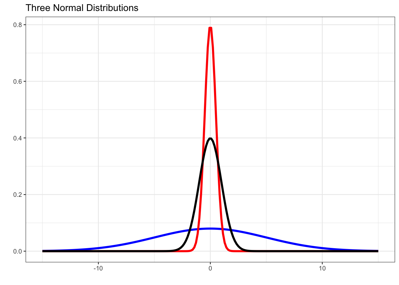
Notice that all three distributions are bell-shaped and are centered at their mean (\(\mu = 0\)). The larger the standard deviation, the shorter and wider the curve, while the smaller the standard deviation, the taller and more narrow the curve.
Given that \(X\sim N\left(\mu, \sigma\right)\), we can compute probabilities associated with observed values of \(X\) by finding the corresponding area beneath the normal curve having mean \(\mu\) and standard deviation \(\sigma\).
Properties of the Normal Distribution: Consider \(X\sim N\left(\mu, \sigma\right)\).
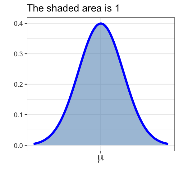
- The area beneath the entire distribution is 1 (since this is equivalent to the probability that \(X\) takes on any of its possible values).
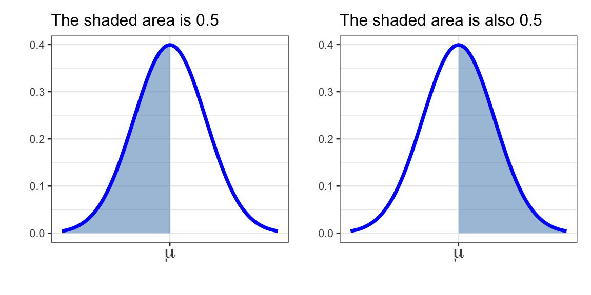
- \(\displaystyle{\mathbb{P}\left[X\leq \mu\right] = \mathbb{P}\left[X\geq \mu\right] = 0.5}\) (the area underneath a full half of the distribution is 0.5)
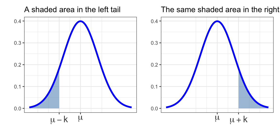
- The distribution is symmetric. In symbols, we write \(\mathbb{P}\left[X\leq \mu - k\right] = \mathbb{P}\left[X \geq \mu + k\right]\) for any \(k\). Geometrically, this means that corresponding lower-tail (left-tail) and upper-tail (right-tail) areas are equal.
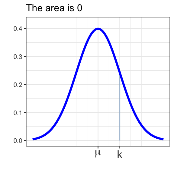
- \(\displaystyle{\mathbb{P}\left[X = k\right] = 0}\) (the probability that \(X\) takes on any prescribed value exactly is \(0\))
Important
Unlike the binomial distribution, where the distinction between at least and more than required careful adjustment, the probability that a continuous variable \(X\) takes on any prescribed value exactly is \(0\) (that is, \(\mathbb{P}\left[X = k\right] = 0\)). This means there is no difference between \(\mathbb{P}\left[X \leq k\right]\) and \(\mathbb{P}\left[X < k\right]\). Similarly, there is no difference between \(\mathbb{P}\left[X \geq k\right]\) and \(\mathbb{P}\left[X > k\right]\).
Sometimes it is useful to be able to estimate probabilities or to estimate the proportion of a population that falls into a range. As long as the population is nearly normal, a convenient set of rough estimates come from the Empirical Rule.
The Empirical Rule
If \(X\sim N\left(\mu, \sigma\right)\), then
- \(\mathbb{P}\left[\mu - \sigma \leq X\leq \mu + \sigma\right] \approx 0.68\) — that is, about 68% of observations lie within one standard deviation of the mean.
- \(\mathbb{P}\left[\mu - 2\sigma \leq X\leq \mu + 2\sigma\right] \approx 0.95\) — that is, about 95% of observations lie within two standard deviations of the mean.
- \(\mathbb{P}\left[\mu - 3\sigma \leq X\leq \mu + 3\sigma\right] \approx 0.997\) — that is, about 99.7% of observations lie within three standard deviations of the mean.
For each of the following, assume that \(X\sim N\left(\mu = 85, \sigma = 5\right)\).
Check Your Understanding: The Empirical Rule I
Use the Empirical Rule to approximate \(\mathbb{P}\left[80\leq X\leq 90\right]\).
Check Your Understanding: The Empirical Rule II
According to the Empirical Rule, which of the following are boundary values for which we expect about 95% of observed values of \(X\) to fall between?
Standardization and \(z\)-Scores
Scenario: Two students, Bob and Sally, are trying to compare how well they did on a college entrance exam. The difficulty comes in that Bob took the SAT which is known to follow an approximate normal distribution with a mean score of 1068 and a standard deviation of 210, while Sally took the ACT which also follows an approximately normal distribution but with a mean score of 20.8 and a standard deviation of 5.8. If Bob scored a 1400 on the SAT and Sally scored a 31 on the ACT, who scored relatively higher?
How do we answer this question? We’ll see two methods.
Method 1: We can standardize the test scores so that they have comparable units.
Definition (z-score): If an observation \(x\) comes from a nearly normal population with mean \(\mu\) and standard deviation \(\sigma\), then we compute the \(z\)-score associated with \(x\) as follows:
\[\displaystyle{z = \frac{x - \mu}{\sigma}}\]
An observation’s \(z\)-score is simply the number of standard deviations it falls above or below the mean.
Try It! Use your spreadsheet to compute Bob and Sally’s \(z\)-scores and answer the questions that follow.
Computing a \(z\)-Score in a Spreadsheet
The \(z\)-score formula is simply arithmetic — no special spreadsheet function is required. In a blank cell, type = followed by the formula \((x - \mu) / \sigma\) using the appropriate values.
For example, to compute Bob’s \(z\)-score, find an empty cell, type =(1400-1068)/210 into it, and press Enter. Compute Sally’s \(z\)-score the same way using her ACT score (31), the ACT mean (20.8), and the ACT standard deviation (5.8).
Be sure to label each result so you remember which \(z\)-score belongs to which student.
Check Your Understanding: \(z\)-Scores I
Which of the following is the \(z\)-score corresponding to Bob? (round to two decimal places)
Check Your Understanding: \(z\)-Scores II
Which of the following is the \(z\)-score corresponding to Sally? (round to two decimal places)
Check Your Understanding: \(z\)-Scores III
Who did relatively better on their standardized exam, Bob or Sally? Why?
A Recap on \(z\)-Scores
We can use \(z\)-scores as a common unit for comparing observations from completely different populations (such as SAT scores and ACT scores). Here’s a recap of the most important information so far:
- If an observation \(x\) comes from a nearly normal population with mean \(\mu\) and standard deviation \(\sigma\), we can compute its \(z\)-score using the formula: \(\displaystyle{z = \frac{x - \mu}{\sigma}}\).
- A \(z\)-score measures the number of standard deviations which an observation falls above or below the mean.
- A positive \(z\)-score means that an observation was above the mean.
- A negative \(z\)-score means that an observation was below the mean.
- The larger a \(z\)-score is in absolute value, the further the corresponding observation falls from the mean.
Method 2: We can compute the percentile corresponding to Bob’s SAT score and the percentile corresponding to Sally’s ACT score.
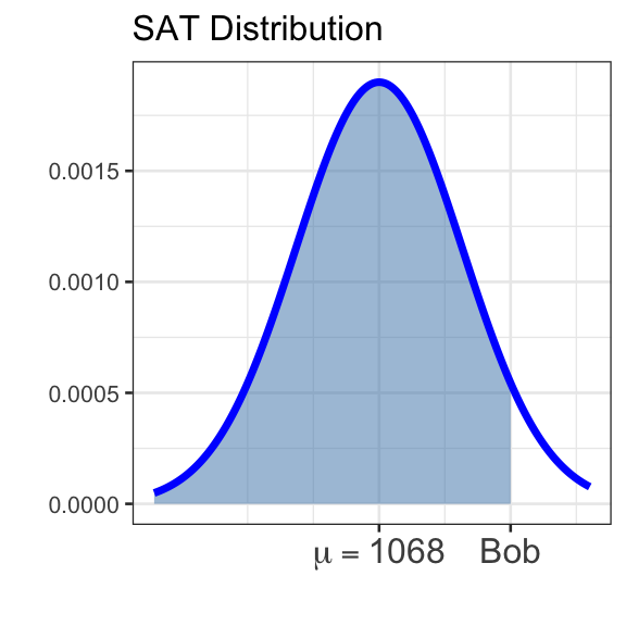
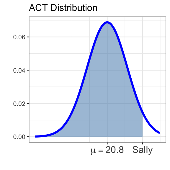
Definition (percentile): Given an observation \(x\) from a population, the percentile corresponding to \(x\) is the proportion of the population which falls at or below \(x\).
In the images below, Bob’s percentile is shown as the shaded area in the distribution on the left, while Sally’s is shown in the distribution on the right.
Computing Percentiles in a Spreadsheet
In Excel and Google Sheets, the NORM.DIST() function computes the area to the left of a given boundary value — that is, the percentile. It takes four arguments:
- The boundary value (\(q\))
- The mean of the distribution (\(\mu\))
- The standard deviation (\(\sigma\))
TRUE— this tells the function to return the cumulative probability/area rather than the height of the density curve (you’ll always useTRUEas the last argument toNORM.DIST())
So if \(X\sim N\left(\mu, \sigma\right)\), then \(\mathbb{P}\left[X\leq q\right] \approx\) =NORM.DIST(q, mean, sd, TRUE).
For example, Bob’s percentile is calculated by typing =NORM.DIST(1400, 1068, 210, TRUE) into an empty cell in your spreadsheet.
Try It! Use your spreadsheet to compute Bob’s and Sally’s percentiles. In a blank cell, type =NORM.DIST(1400, 1068, 210, TRUE) for Bob. Then adapt the formula to compute Sally’s percentile (her ACT score was 31, the mean was 20.8, and the standard deviation was 5.8). Label both results.
Check Your Understanding: Percentiles I
Which of the following is the percentile corresponding to Bob? (round to four decimal places)
Check Your Understanding: Percentiles II
Which of the following is the percentile corresponding to Sally? (round to four decimal places)
Check Your Understanding: Percentiles III
Who did relatively better on their standardized exam, Bob or Sally? Why?
We’ll make good use of this second method for a while, but don’t forget about standardization and \(z\)-scores — we’ll need that strategy quite often later in our course! For now, let’s move on to practicing with finding probabilities from a normal distribution using NORM.DIST() in your spreadsheet.
Computing Probability from a Normal Distribution
Through this section you’ll get practice finding probabilities by using NORM.DIST() to compute areas in your spreadsheet. Remember that NORM.DIST(q, mean, sd, TRUE) always returns the area to the left of the boundary value q in the distribution with the specified mean and standard deviation.
For these first few questions I’ll draw pictures for you, but you should be prepared to draw your own shortly.
Question 1: Find \(\mathbb{P}\left[Z <\right.\) \(\left.\right]\) — remember that \(Z\sim N\left(\mu = 0, \sigma = 1\right)\).
In your spreadsheet, compute this probability and enter your result below.
Hint 1
Be sure you can answer: “why does the picture to the right correspond to the probability requested?”
Hint 2
The shaded area is everything to the left of the boundary value — that is exactly what NORM.DIST() with TRUE computes.
Hint 3
In a blank spreadsheet cell, type =NORM.DIST( followed by four arguments separated by commas: the boundary value, the mean, the standard deviation, and TRUE. The standard normal distribution has mean 0 and standard deviation 1.
Hint 4 (Solved)
In your spreadsheet, type =NORM.DIST(___, 0, 1, TRUE), where the blank is filled in by , and press Enter. Input the result below.
pnorm(boundary1, 0, 1)
pnorm(boundary1, 0, 1)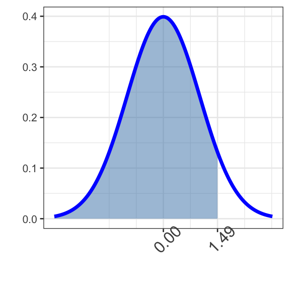
Question 2: Find \(\mathbb{P}\left[Z <\right.\) \(\left.\right]\).
In your spreadsheet, compute this probability and enter your result below.
Hint 1
Would you be able to draw the picture if I hadn’t provided it? Try practicing this picture-drawing skill — it will serve you well.
Hint 2
How “big” do you expect this probability to be? Should it be more than 0.5 or less than 0.5?
Hint 3
Since the boundary value is negative and the distribution is symmetric around 0, the shaded area covers less than half of the distribution — so the answer should be less than 0.5. NORM.DIST() with TRUE will give you the area to the left of your boundary directly.
Hint 4 (Solved)
In your spreadsheet, type =NORM.DIST(___, 0, 1, TRUE), with the blank filled in by and press Enter. Input the result below.
pnorm(boundary2, 0, 1)
pnorm(boundary2, 0, 1)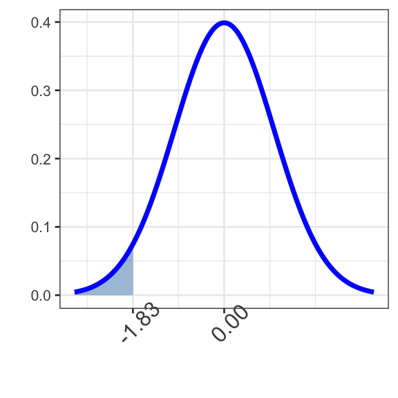
Question 3: Find \(\mathbb{P}\left[Z >\right.\) \(\left.\right]\).
In your spreadsheet, compute this probability and enter your result below.
Hint 1
This one is different from the previous two — the shaded area is to the right of the boundary value. NORM.DIST() with TRUE always gives the area to the left, so you’ll need to think about how to use it here.
Hint 2
The total area under the normal curve is 1. If you compute the area to the left of and subtract it from 1, you’ll be left with the area to the right — which is what you want.
Hint 3 (Solved)
In your spreadsheet, type =1-NORM.DIST(___, 0, 1, TRUE), where the blank is filled in by , and press Enter. Input the result below.
1 - pnorm(boundary3, 0, 1)
1 - pnorm(boundary3, 0, 1)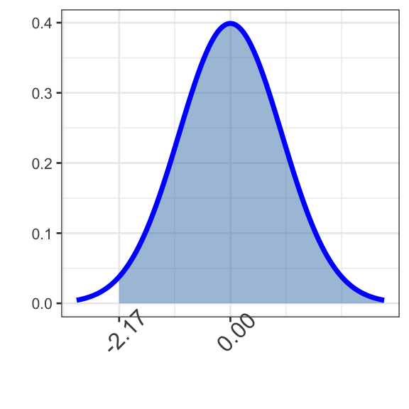
Question 4: Find \(\mathbb{P}\left[Z >\right.\) \(\left.\right]\).
In your spreadsheet, compute this probability and enter your result below.
Hint 1
Use the same approach as Question 3 — subtract the left-tail area from 1.
Hint 2
How large do you expect the answer to be?
Hint 3
The boundary is positive and to the right of the mean, so the right-tail area should be less than 0.5.
Hint 4 (Solved)
In your spreadsheet, type =1-NORM.DIST(___, 0, 1, TRUE), with the blank filled in by and press Enter. Input the result below.
1 - pnorm(boundary4, 0, 1)
1 - pnorm(boundary4, 0, 1)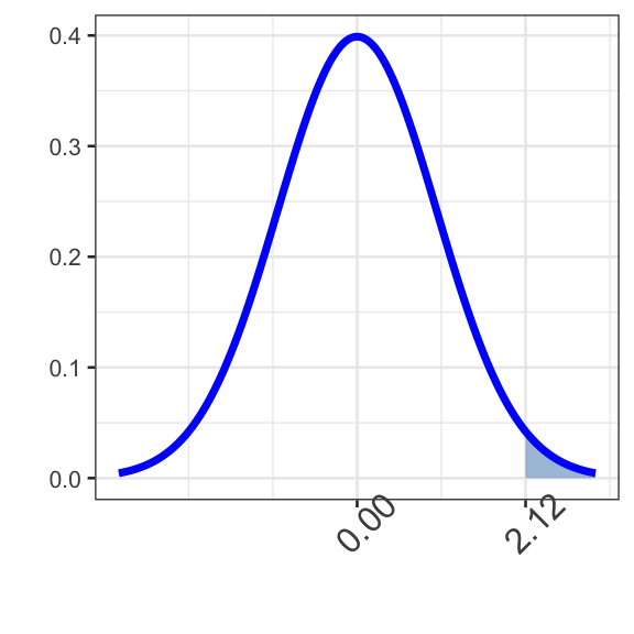
Question 5: Find \(\mathbb{P}\left[\right.\) \(< Z <\) \(\left.\right]\).
In your spreadsheet, compute this probability and enter your result below.
Hint 1
The shaded area sits between two boundary values. A single NORM.DIST() call won’t get you there directly — you’ll need two calls and combine them.
Hint 2
Start with the cumulative area up to the upper boundary ( ) — that’s larger than what you want because it includes area to the left of as well. Subtract the area to the left of the lower boundary to remove the unwanted part.
Hint 3 (Solved)
In your spreadsheet, type =NORM.DIST(___, 0, 1, TRUE) - NORM.DIST(___, 0, 1, TRUE), where the first blank is filled in by and the second by , and press Enter. Input the result below.
pnorm(boundary5b, 0, 1) - pnorm(boundary5a, 0, 1)
pnorm(boundary5b, 0, 1) - pnorm(boundary5a, 0, 1)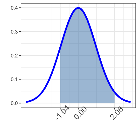
Question 6: Find \(\mathbb{P}\left[Z <\right.\) \(\text{ or } Z >\) \(\left.\right]\).
In your spreadsheet, compute this probability and enter your result below.
Hint 1
There are two separate shaded regions — a left tail and a right tail. Compute each area separately and add them together.
Hint 2
The left-tail area (below ) comes directly from NORM.DIST() with TRUE. The right-tail area (above ) requires the subtract-from-one approach.
Hint 3 (Solved)
In your spreadsheet, type =NORM.DIST(___, 0, 1, TRUE) + (1-NORM.DIST(___, 0, 1, TRUE)), with the first blank filled in by and the second filled in by , and press Enter. Input the result below.
pnorm(boundary6a, 0, 1) + (1 - pnorm(boundary6b, 0, 1))
pnorm(boundary6a, 0, 1) + (1 - pnorm(boundary6b, 0, 1))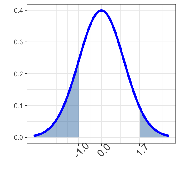
Question 7: Find \(\mathbb{P}\left[\left|Z\right| >\right.\) \(\left.\right]\).
In your spreadsheet, compute this probability and enter your result below.
Hint 1
Recall that \(|Z|\) denotes the absolute value of \(Z\), which measures distance from 0. We are interested in values of \(Z\) whose distance from 0 exceeds — so the shaded region is two tails, symmetric around 0.
Hint 2
You could use the same approach as Question 6. But because the distribution is symmetric, the two tail areas are equal — so you can compute just the left-tail area and double it, which is a little simpler.
Hint 3 (Solved)
The left-tail boundary is (the negative version of ). In your spreadsheet, type =2*NORM.DIST(___, 0, 1, TRUE), where the blank is filled in by , and press Enter. Input the result below.
2 * pnorm(-boundary7, 0, 1)
2 * pnorm(-boundary7, 0, 1)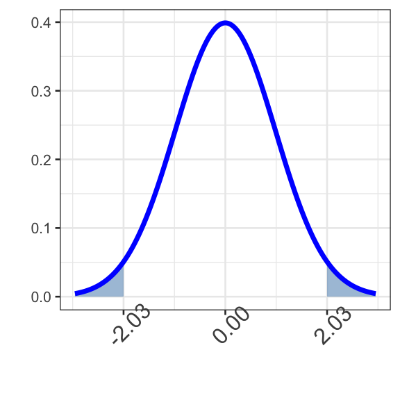
Probabilities from Other Normal Distributions
Through the last seven problems you only worked with the standard normal distribution — \(Z\sim N\left(\mu = 0, \sigma = 1\right)\). You can find probabilities from any normal distribution using NORM.DIST() — just supply the appropriate mean and standard deviation as the second and third arguments instead of 0 and 1.
Finding Percentile Cutoffs on a Normal Distribution
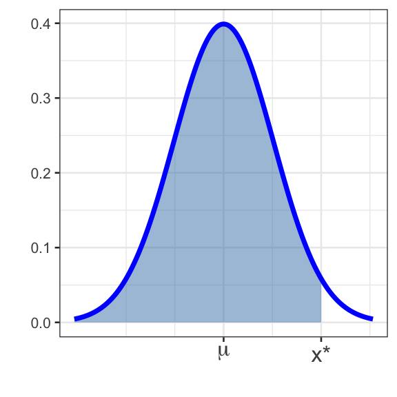
Recall from earlier that the \(p^{th}\) percentile of a random variable \(X\) is the value \(x^*\) such that \(\mathbb{P}\left[X < x^*\right] = p\).
If \(X\sim N\left(\mu, \sigma\right)\), we can find the cutoff \(x^*\) for which \(\mathbb{P}\left[X < x^*\right] = p\) using the NORM.INV() function in your spreadsheet. The NORM.INV() function takes three arguments: the area to the left of the desired cutoff (\(p\)), the mean, and the standard deviation.
So the \(p^{th}\) percentile of \(X\) is given by =NORM.INV(p, mean, sd).
Recall that SAT scores follow \(N\left(\mu = 1068, \sigma = 210\right)\) and ACT scores follow \(N\left(\mu = 20.8, \sigma = 5.8\right)\).
Try It! In your spreadsheet, you can use NORM.INV() to find the minimum SAT score required to fall in the 95th percentile by finding an empty cell and entering =NORM.INV(0.95, 1068, 210). Check the result and then adapt the formula to find the minimum ACT score required to fall into the top 10% of all ACT test takers. Enter your result for the ACT cutoff below.
Hint 1
The arguments to NORM.INV() are, in order: the area to the left of the desired cutoff, the mean of the normal distribution, and the standard deviation.
Hint 2
To be in the top 10% of ACT scores, a student must score higher than 90% of all test takers — so the area to the left of the cutoff is 0.90. The ACT mean is 20.8 and the standard deviation is 5.8.
Hint 3(Solved)
In your spreadsheet, type =NORM.INV(0.90, 20.8, 5.8) and press Enter. Input the resulting value below.
qnorm(0.9, 20.8, 5.8)
qnorm(0.9, 20.8, 5.8)Practice with the Normal and Binomial Distributions
Through this last section you’ll work through a set of problems, some of which use the normal distribution while others use the binomial distribution. It is up to you to determine which distribution should be applied in each problem. Below are a few helpful reminders:
Binomial and Normal Distributions — Spreadsheet Functions Recap
- The binomial distribution can be applied to scenarios of repeated trials where each trial has two possible outcomes and the probability of “success” on each trial remains constant. If \(X\) is the number of successes in a binomial experiment with \(n\) trials and probability of success \(p\):
- \(\mathbb{P}\left[X = k\right] \approx\)
=BINOM.DIST(k, n, p, FALSE) - \(\mathbb{P}\left[X \leq k\right] \approx\)
=BINOM.DIST(k, n, p, TRUE)
- \(\mathbb{P}\left[X = k\right] \approx\)
- The normal distribution can be applied to scenarios where data follow at least a nearly-normal distribution. If \(X\sim N\left(\mu, \sigma\right)\):
- \(\mathbb{P}\left[X \leq k\right] \approx\)
=NORM.DIST(k, mean, sd, TRUE) - The \(p^{th}\) percentile of \(X\) is given by
=NORM.INV(p, mean, sd)
- \(\mathbb{P}\left[X \leq k\right] \approx\)
Practice Problem 1: The National Vaccine Information Center estimates that 90% of Americans have had chickenpox by the time they reach adulthood. Suppose we take a random sample of American adults. Answer each of the following, making use of your spreadsheet functionality where appropriate.
- Compute the expected number of adults in our sample who will have had chickenpox. Enter your result below.
Hint 1
Is this scenario best-modeled by a binomial distribution or a normal distribution?
Hint 2
There are adults being surveyed, they are from a random sample (independent), and each is being asked a yes/no question — “have you had chickenpox?” This fits the assumptions of a binomial experiment.
Hint 3 (Solved)
The expected value of a binomial random variable is \(\mathbb{E}[X] = n \cdot p\), where \(n\) is the number of trials and \(p\) is the probability of success. In your spreadsheet, type = 68*0.90 and press Enter. Input the result in the code cell.
chickPoxSampSize * 0.90
chickPoxSampSize * 0.90- Compute the standard deviation in number of adults who will have had chickenpox across samples of size . Enter your result below.
Hint 1
The standard deviation of a binomial random variable is \(s_X = \sqrt{n \cdot p \cdot (1 - p)}\). Here \(n\) = and \(p\) = 0.90. Use SQRT() in your spreadsheet.
Hint 2 (Solved)
In your spreadsheet, type =SQRT(68*0.90*(1-0.90)) and press Enter. Input the resulting value.
sqrt(chickPoxSampSize * 0.9 * 0.1)
sqrt(chickPoxSampSize * 0.9 * 0.1)
Check Your Understanding: Surprising Results?
Would you be surprised if your sample of adults contained at most adults who have had chickenpox? Why? Select all that are appropriate.
While you answer the following questions, it might be useful to refer back to the example and solution document from the Topic 5 activity.
- Find the probability that exactly adults in your sample of will have had chickenpox. Enter your result below.
Hint 1
We are still working with a binomial scenario. Since we want exactly a specific number of successes, use BINOM.DIST() with FALSE as the last argument.
Hint 2
The four arguments are: the number of successes you are interested in ( ), the sample size ( ), the probability of success ( 0.90 ), and FALSE.
Hint 3
In your spreadsheet, type =BINOM.DIST(___, ___ , 0.90, FALSE), where the first blank is filled in by and the second by , and press Enter. Input the result.
dbinom(chickPox_exact1, chickPoxSampSize, 0.9)
dbinom(chickPox_exact1, chickPoxSampSize, 0.9)- Find the probability that exactly adults in your sample of will not have had chickenpox. Enter your result below.
Hint 1
Read carefully — this question asks about adults who have not had chickenpox. That changes both the count of interest and the probability argument.
Hint 2
The probability of a single adult not having had chickenpox is 1 - 0.90 = 0.10. The number of adults who have not had chickenpox is and the sample size is .
Hint 3 (Solved)
In your spreadsheet, type =BINOM.DIST(___, ___, 0.10, FALSE), where the first blank is filled in by and the second by , and press Enter. Input the result.
dbinom(chickPox_exact2, chickPoxSampSize, 0.1)
dbinom(chickPox_exact2, chickPoxSampSize, 0.1)- Find the probability that at most adults in your sample of will have had chickenpox. Enter your result below.
Hint 1
“At most” covers a range of outcomes (0, 1, 2, … up to ). Use BINOM.DIST() with TRUE as the last argument.
Hint 2 (Solved)
In your spreadsheet, type =BINOM.DIST(___, ___, 0.90, TRUE), where the first blank is filled in by and the second by , and press Enter. Input the result.
pbinom(chickPox_atmost, chickPoxSampSize, 0.9)
pbinom(chickPox_atmost, chickPoxSampSize, 0.9)- Find the probability that at least adults in your sample of will have had chickenpox. Enter your result below.
Hint 1
BINOM.DIST() with TRUE computes the probability of at most some number of successes — not at least. Draw a picture to start.
Hint 2
BINOM.DIST() with TRUE computes the probability of at most some number of successes — not at least. Draw a picture to start. You’ll need the “subtract from 1” approach here.
Hint 3
To get “at least ”, subtract the probability of “at most ” from 1.
Hint 4 (Solved)
To get “at least ”, subtract the probability of “at most ” from 1. In your spreadsheet, type =1-BINOM.DIST(___, ___, 0.90, TRUE), where the first blank is filled in by and the second by , and press Enter. Input the result.
1 - pbinom(chickPox_atleast - 1, chickPoxSampSize, 0.9)
1 - pbinom(chickPox_atleast - 1, chickPoxSampSize, 0.9)- Find the probability that more than but less than adults in your sample of will have had chickenpox. Enter your result below.
Hint 1
Multiple outcomes are of interest, so use BINOM.DIST() with TRUE. Draw a picture — you’ll need two calls, one for the upper boundary and one to subtract out the outcomes below the lower boundary.
Hint 2
The phrase “more than but less than ” means both boundaries are excluded. The upper call covers outcomes up through ; the lower call removes outcomes up through .
Hint 3
In your spreadsheet, type =BINOM.DIST(___, 68, 0.90, TRUE) - BINOM.DIST(___, 68, 0.90, TRUE). What should you use in place of the first blank inside of each call to BINOM.DIST()?
Hint 4 (Solved)
In your spreadsheet, type =BINOM.DIST(___, 68, 0.90, TRUE) - BINOM.DIST(___, 68, 0.90, TRUE)Z. The first blanks are filled in by and , respectively, and press Enter. Input the result.
pbinom(chickPox_between_hi - 1, chickPoxSampSize, 0.9) - pbinom(chickPox_between_lo, chickPoxSampSize, 0.9)
pbinom(chickPox_between_hi - 1, chickPoxSampSize, 0.9) - pbinom(chickPox_between_lo, chickPoxSampSize, 0.9)Practice Problem 2: Sophia took the Graduate Record Examination (GRE) and scored 160 on the Verbal Reasoning section and 157 on the Quantitative Reasoning section. The mean score on the Verbal Reasoning section for all test takers was 151 with a standard deviation of 7, and the mean score for the Quantitative Reasoning section was 153 with a standard deviation of 7.67. Suppose we can assume that both score distributions are nearly normal.
- Use your spreadsheet to compute Sophia’s \(z\)-score on the Quantitative Reasoning exam. Enter your result below.
Hint 1
The \(z\)-score formula is \((x - \mu) / \sigma\). No special function is needed — just type the arithmetic directly into a spreadsheet cell.
Hint 2
Sophia scored 157 on the Quantitative Reasoning exam, the mean is 153, and the standard deviation is 7.67. In your spreadsheet, type =(157-153)/7.67 and press Enter. Enter the result below.
(157 - 153) / 7.67
(157 - 153) / 7.67- Use your spreadsheet to compute Sophia’s \(z\)-score on the Verbal Reasoning exam. Enter your result below.
Hint 1
Use the same approach as above. Sophia scored 160 on the Verbal Reasoning exam, the mean is 151, and the standard deviation is 7. In your spreadsheet, type =(160-151)/7 and press Enter.
(160 - 151) / 7
(160 - 151) / 7
Check Your Understanding: Comparing \(z\)-Scores
What do these \(z\)-scores tell you?
- Find the proportion of test takers that Sophia scored higher than on the Quantitative Reasoning exam (that is, find her percentile). Enter your result below.
Hint 1
Scores are approximately normally distributed, so use NORM.DIST(). We want the proportion of test takers below Sophia’s score — that’s the area to the left, which is exactly what NORM.DIST() with TRUE gives.
Hint 2
Sophia’s Quantitative Reasoning score is 157, the mean is 153, and the standard deviation is 7.67. In your spreadsheet, type =NORM.DIST(157, 153, 7.67, TRUE) and press Enter. Enter the result below.
pnorm(157, 153, 7.67)
pnorm(157, 153, 7.67)- Find the proportion of test takers doing better than Sophia on the Verbal Reasoning exam. Enter your result below.
Hint 1
We want the area to the right of Sophia’s score — the proportion scoring higher than her. Use the subtract-from-one approach.
Hint 2
Sophia’s Verbal Reasoning score is 160, the mean is 151, and the standard deviation is 7. In your spreadsheet, type =1-NORM.DIST(160, 151, 7, TRUE) and press Enter. Enter the result below.
1 - pnorm(160, 151, 7)
1 - pnorm(160, 151, 7)Submit
If you are part of a course with an instructor who is grading your work on these activities, please copy and submit both of the hashes below using the method your instructor has requested.
Question Hash
The hash below encodes your responses to the multiple choice and checkbox questions in this activity.
Exercise Hash
Click the button below to generate your exercise submission code. This hash encodes your work on the graded exercises in this activity.
You must have attempted the graded exercises before clicking — clicking generates a snapshot of your current results. If you have completed the activity over multiple sessions, please go back through and enter your answer in each graded exercise cell before generating the hash below, to ensure your most recent results are recorded.
Summary
Main Takeaways
- A normal distribution is bell-shaped and fully described by its mean \(\mu\) and standard deviation \(\sigma\), written \(N(\mu, \sigma)\). Larger \(\sigma\) produces a shorter, wider curve; smaller \(\sigma\) produces a taller, narrower curve.
- The Empirical Rule for data following \(N(\mu, \sigma)\) states that approximately 68% of observations fall within one standard deviation of the mean, 95% within two, and 99.7% within three.
- For a continuous distribution, \(\mathbb{P}[X = k] = 0\), so there is no distinction between strict (\(<\), \(>\)) and non-strict (\(\leq\), \(\geq\)) inequalities when computing probabilities.
- A \(z\)-score measures how many standard deviations an observation falls from the mean: \(z = (x - \mu)/\sigma\). In a spreadsheet, compute it as
=(x-mean)/sd. Converting raw observed values to \(z\)-scores allow comparison across different normal distributions on a common scale. =NORM.DIST(q, mean, sd, TRUE)returns the area to the left of \(q\) — that is, \(\mathbb{P}[X \leq q]\). For right-tail and two-tail probabilities, draw a picture to inform how to use and combine calls toNORM.DIST()in order to find desired probabilities.=NORM.INV(p, mean, sd)returns the value \(x^*\) such that \(\mathbb{P}[X \leq x^*] = p\). This is called the \(p^{th}\) percentile. Remember that \(p\) must be the area to the left of the desired cutoff.- When a scenario involves repeated independent yes/no trials with constant probability, use the binomial distribution (
BINOM.DIST()). When data are approximately normally distributed, use the normal distribution (NORM.DIST(),NORM.INV()).