Topic 3: Descriptive Statistics for Numerical and Categorical Data

function ok_checkbox(response, n) {
  if (!response || response.length === 0)
    return html`<span style="color:purple">You haven't answered yet.</span>`;
  if (response.toString() === n)
    return html`<span style="color:green">Correct ✓</span>`;
  return html`<span style="color:red">Not Yet! ✗</span>`;
}

mutable ok_response = (response, n) => { return html`Loading...` };

About

This activity builds off of what we learned in the Topic 1 and Topic 2 activities. We’ll learn how to use R to analyse numeric and categorical data. We discuss and implement measures of central tendency and spread (including inquiry into robustness in the presence of outliers) for numerical data, and measures of frequency for categorical data.

Descriptive Statistics

Workbook Objectives: This workbook covers the following objectives.

• Compute and discuss appropriate summaries for both numerical and categorical data
• Regarding numerical variables, discuss the difference between mean and median as well as standard deviation and inter-quartile range. Identify when each measure is appropriate.
• Compute summary statistics both by hand and with the use of R

Important Reminders: The following previously mastered material is necessary for success through this workbook.

• A variable is numerical if a summary statistic such as the mean has a meaningful interpretation.
• A variable is categorical if it serves to sort observations into different groups (categories).
• The unique values which a variable takes are called the levels of that variable.

Summarizing Numerical (Quantitative) Data

Recall: Variables for which computation of measures like the mean (average) or standard deviation are meaningful are numerical variables.

Measuring Central Tendency

Measures of Central Tendency (Averages): The mean and median both attempt to measure the center of a dataset.

• The mean of a set of observations is the traditional average. We typically denote the mean by \(\bar{x}\) (or \(\mu\) in the case of population-level data) and it is computed as follows: \[\bar{x} = \frac{\displaystyle{\sum_{i=1}^{n}{x_i}}}{n} = \frac{x_1+x_2+x_3+\cdots+x_n}{n}\]

• The median is the middle value for a set of observations. To compute the median, list the numbers in ascending order and find the number or numbers in the middle of the list. In the case that there is a single middle number, that is the median. In the case where there are two middle numbers, we take the mean of those two.

Example: The following are three random samples of carat values from the diamonds dataset.

Sample_One	Sample_Two	Sample_Three
0.41	2.68	1.05
1.01	1.01	0.31
1.22	0.26	0.31
1.02	0.90	0.30
0.30	0.43	0.40
0.30	0.53	1.50
1.00	2.00	2.27
1.17	0.33	10.00

1. Use the code block below to compute the mean of Sample_One.

Hint 1

Manually add up the carat values in Sample One, and then divide by the total number of diamonds in the sample.

______

Hint 2

Manually add up the carat values in Sample One, and then divide by the total number of diamonds in the sample. Fill in the blanks.

(___ + ___ + ___ + ___ + ___ + ___ + ___ + ___) / ___

Hint 3 (Solved)

Manually add up the carat values in Sample One, and then divide by the total number of diamonds in the sample.

(0.41 + 1.01 + 1.22 + 1.02 + 0.30 + 0.30 + 1.00 + 1.17) / 8

(0.41 + 1.01 + 1.22 + 1.02 + 0.30 + 0.30 + 1.00 + 1.17) / 8

(0.41 + 1.01 + 1.22 + 1.02 + 0.30 + 0.30 + 1.00 + 1.17) / 8

In R we can easily compute the means and medians for our samples or for the entire data set! You might remember from our most recent notebook that the $ operator can be used to access an entire column of a data frame. I’ve stored the samples in a data frame called samples. R includes a function mean() for computing the mean of a list of numbers and a function median() for computing the median. The following methods both compute the mean() of Sample_Two.

mean(samples$Sample_Two)

[1] 1.0175

samples |>
  summarize(avg_carat_wt = mean(Sample_Two))

  avg_carat_wt
1       1.0175

While the second method involves more typing, it is much more readable. Getting used to using the pipe operator (|>) will allow us to chain data manipulation operations together, resulting in very readable analyses.

2. Use the code block below so that it computes the mean of Sample_Three. You may use whichever method you prefer here.

Hint 1

Start with the code below (copied from our earlier code chunk) and update it to compute the mean of Sample_Three.

samples |>
  summarize(avg_carat_wt = mean(Sample_Two))

Hint 2

Start with the code below (copied from our earlier code chunk) and update it to compute the mean of Sample_Three.

samples |>
  summarize(avg_carat_wt = mean(___))

Hint 3 (Solved)

Start with the code below (copied from our earlier code chunk) and update it to compute the mean of Sample_Three.

samples |>
  summarize(avg_carat_wt = mean(Sample_Three))

samples |> summarize(avg_carat_wt = mean(Sample_Three))

samples |>
  summarize(avg_carat_wt = mean(Sample_Three))

3. Use the median() function and the code block below to compute the median of each of the samples and then answer the question that follows. (Note. There are several ways to obtain the medians, so this code block won’t evaluate you as correct/incorrect.)

Hint 1

Start with the copied code again, and update it to compute the median instead of the mean.

samples |>
  summarize(avg_carat_wt = mean(Sample_Two))

Hint 2

Start with the copied code again, and update it to compute the median instead of the mean.

samples |>
  summarize(avg_carat_wt = ___(Sample_Two))

Hint 3

Power move! The summarize() function can compute multiple summary statistics at once. Update the code below to compute all three medians at once.

samples |>
  summarize(
    avg_carat_wt_samp1 = mean(Sample_One),
    avg_carat_wt_samp2 = mean(Sample_Two),
    avg_carat_wt_samp3 = mean(Sample_Three)
  )

Hint 4

Power move! The summarize() function can compute multiple summary statistics at once. Update the code below to compute all three medians at once.

samples |>
  summarize(
    median_carat_wt_samp1 = ___(Sample_One),
    median_carat_wt_samp2 = ___(Sample_Two),
    median_carat_wt_samp3 = ___(Sample_Three)
  )

Hint 5 (Solved)

Power move! The summarize() function can compute multiple summary statistics at once. Update the code below to compute all three medians at once.

samples |>
  summarize(
    median_carat_wt_samp1 = median(Sample_One),
    median_carat_wt_samp2 = median(Sample_Two),
    median_carat_wt_samp3 = median(Sample_Three)
  )

Check Your Understanding: Measures of Center

What does your work above tell you about the mean and median as measures of central tendency?

viewof q1 = Inputs.radio(
  new Map([
    ["The mean is generally larger than the median.", 1],
    ["The mean is generally smaller than the median.", 2],
    ["The mean is usually close to the median.", 3],
    ["The mean is more strongly distorted by outliers (unusually large or small observed values) than the median is.", 4]
  ]),
  {value: JSON.parse(localStorage.getItem("q1_selected") ?? "null")}
);

{

  localStorage.setItem("q1_selected", JSON.stringify(q1));
  localStorage.setItem("q1_correct", "4");
  localStorage.setItem("q1_result", q1 === null ? "unattempted" : (q1 == 4 ? "correct" : "incorrect"));

}

ok_response(q1, "4");

4. In our first notebook we saw that we can use sample data to make generalizations about populations for which the sample is representative. Answer the following questions with this in mind.

Check Your Understanding: Sampling and Validity I

Assuming that the samples of diamonds were taken randomly, which of the following claims is justified?

viewof q2 = Inputs.radio(
  new Map([
    ["The mean from Sample_Three is too high.", 1],
    ["The mean from Sample_One is too low.", 2],
    ["Each of the sample means provides an estimate for the population mean.", 3],
    ["The population mean is equal to the sample means.", 4]
  ]),
  {value: JSON.parse(localStorage.getItem("q2_selected") ?? "null")}
);

{
  localStorage.setItem("q2_selected", JSON.stringify(q2));
  localStorage.setItem("q2_correct", "3");
  localStorage.setItem("q2_result", q2 === null ? "unattempted" : (q2 == 3 ? "correct" : "incorrect"));

}

ok_response(q2, "3");

Check Your Understanding: Sampling and Validity II

Which of the following would result in improved estimates for the true mean carat weight of diamonds in our population? Select all that apply.

viewof q3 = Inputs.checkbox(
  new Map([
    ["Take the mean of the sample means.", 1],
    ["Combine the three samples into a single sample of 24 diamonds (rather than three separate samples of 8), and take its mean.", 2],
    ["Take samples using smaller sample sizes.", 3],
    ["Stratify the diamonds according to price (low, medium, and high) and take a random sample of diamonds of each price category.", 4],
    ["Take samples including more diamonds.", 5]
  ]),
  {value: JSON.parse(localStorage.getItem("q3_selected") ?? "[]") ?? []}
);

{
  
  localStorage.setItem("q3_selected", JSON.stringify(q3));
  localStorage.setItem("q3_correct", "1,2,5");
  localStorage.setItem("q3_result", (!q3 || q3.length === 0) ? "unattempted" : (q3.toString() === "1,2,5" ? "correct" : "incorrect"));

}

ok_checkbox(q3, "1,2,5");

Aside: Defining Our Own Data

For data which is not already known to R (i.e. data which is not part of a data frame), we can still use R to quickly perform computations. Consider the distributions of doors knocked on by two political campaign workers last week (Monday – Friday): \(\begin{array}{lcl} \text{Worker A} & : & 23,~24,~25,~26,~27\\ \text{Worker B} & : & 0,~15,~25,~35,~50\end{array}\). We do this below with the help of the c() function in R, which can be used to create lists of values.

The following code block finds the mean and median for Worker A — execute the code block to find the mean and median. Once you’ve done this for Worker A, add two lines to the bottom of the code block so that it also finds the mean and median for Worker B.

Hint 1

Copy and paste the two existing lines and replace the data inside of c() to reflect Worker B in the last two lines.

mean(c(23, 24, 25, 26, 27))
median(c(23, 24, 25, 26, 27))

Hint 1

Copy and paste the two existing lines and replace the data inside of c() to reflect Worker B in the last two lines.

# Worker A
mean(c(23, 24, 25, 26, 27))
median(c(23, 24, 25, 26, 27))

# Worker B
mean(c(___))
median(c(___))

Hint 3 (Solved)

Copy and paste the two existing lines and replace the data inside of c() to reflect Worker B in the last two lines.

# Worker A
mean(c(23, 24, 25, 26, 27))
median(c(23, 24, 25, 26, 27))

# Worker B
mean(c(0, 15, 25, 35, 50))
median(c(0, 15, 25, 35, 50))

mean(c(23, 24, 25, 26, 27)) median(c(23, 24, 25, 26, 27)) mean(c(0, 15, 25, 35, 50)) median(c(0, 15, 25, 35, 50))

mean(c(23, 24, 25, 26, 27))
median(c(23, 24, 25, 26, 27))
mean(c(0, 15, 25, 35, 50))
median(c(0, 15, 25, 35, 50))

5. Use your explorations of the means and medians for the campaign workers to answer the following question.

Check Your Understanding: Measures of Center

Which of the following are correct? Select all that apply.

viewof q4 = Inputs.checkbox(
  new Map([
    ["Worker A and Worker B had the same mean and median number of doors knocked.", 1],
    ["Worker A and Worker B had identical door-knocking strategies.", 2],
    ["Measures of center alone are not enough to describe numerical data.", 3]
  ]),
  {value: JSON.parse(localStorage.getItem("q4_selected") ?? "[]") ?? []}
);

{
  localStorage.setItem("q4_selected", JSON.stringify(q4));
  localStorage.setItem("q4_correct", "1,3");
  localStorage.setItem("q4_result", (!q4 || q4.length === 0) ? "unattempted" : (q4.toString() === "1,3" ? "correct" : "incorrect"));
  
}

ok_checkbox(q4, "1,3");

Measuring Spread

Measures of Variability: Clearly, the center of a dataset doesn’t tell the entire story. Our two political campaign workers obviously have very different door-knocking strategies but both have a mean (and median) of 25 doors per day. We should also measure the spread of data.

The standard deviation of a set of observations is denoted by \(s\) (or \(\sigma\) in the case of population-level data) and is computed as follows: \[s = \sqrt{\frac{\displaystyle{\sum_{i=1}^{n}{\left(x_i-\bar{x}\right)^2}}}{n-1}}\]

We should also note that if you are certain that you are working with population-level data, then the denominator used to compute the standard deviation should be changed to \(N\) (the population size). We can do this because there is no uncertainty in estimating the population standard deviation if we have records from every element of the population.

Explaining the Standard Deviation Formula: The standard deviation seeks to measure an “average deviation” from the mean.

• If we don’t look too closely at the formula, we can see the summation symbol \(\left(\sum\right)\) as well as division (by just about the number of values we’ve added up). That’s almost like an average!
• What are we averaging? The quantity \(\left(x - \bar{x}\right)\) denotes an observed value’s deviation from the mean. We shouldn’t average these values though, because since the mean sits in the center of the data and we would have deviations above the mean (positive) “cancelling out” deviations below the mean (negative).
• We square the deviations which has two effects: (i) all of the squared deviations are now non-negative, so that no cancellation can occur, and (ii) large deviations from the mean carry a larger weight in measuring the standard deviation.
• Since we squared the deviations before computing the “average”, the units of measure are no longer comparable to the original units that the variable was measured in — the units are square units now. This is why we see the large square root as the last piece of the formula — taking the square root brings us back to the original units.

The inter-quartile range (IQR) of a set of observations measures the spread of the “middle 50 percent” of the observations. The IQR is the distance between \(Q_1\) (the 25th percentile) and \(Q_3\) (the 75th percentile).

• Note that the median of a set of observations splits the set into two halves: an upper half and a lower half. The median of the lower half is called the first quartile (\(Q_1\)) while the median of the upper half is called the third quartile (\(Q_3\)). The interquartile range is the distance between \(Q_1\) and \(Q_3\). That is, \[IQR = Q_3 - Q_1\]

6. Check your intuition about the standard deviation and interquartile range by answering the questions below.

Check Your Understanding: Measures of Spread I

Without carrying out the computations, which of the samples of diamonds has the largest standard deviation?

viewof q5 = Inputs.radio(
  new Map([
    ["Sample One", 1],
    ["Sample Two", 2],
    ["Sample Three", 3]
  ]),
  {value: JSON.parse(localStorage.getItem("q5_selected") ?? "null")}
);

{

  localStorage.setItem("q5_selected", JSON.stringify(q5));
  localStorage.setItem("q5_correct", "3");
  localStorage.setItem("q5_result", q5 === null ? "unattempted" : (q5 == 3 ? "correct" : "incorrect"));

}

ok_response(q5, "3");

Check Your Understanding: Measures of Spread II

Which measure of spread is more greatly impacted by the presence of outliers?

viewof q6 = Inputs.radio(
  new Map([
    ["Standard Deviation", 1],
    ["Interquartile Range", 2]
  ]),
  {value: JSON.parse(localStorage.getItem("q6_selected") ?? "null")}
);

{
  localStorage.setItem("q6_selected", JSON.stringify(q6));
  localStorage.setItem("q6_correct", "1");
  localStorage.setItem("q6_result", q6 === null ? "unattempted" : (q6 == 1 ? "correct" : "incorrect"));

}

ok_response(q6, "1");

The two plots below are a histogram (left) and a boxplot (right), each showing the distribution of carat weights for the diamonds in our population.

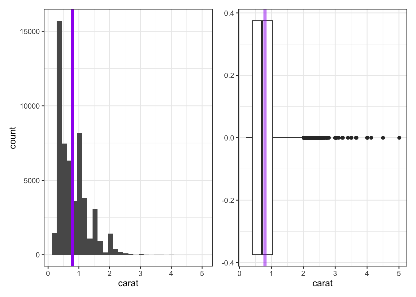
• The histogram does a nice job showing the true shape of the data, but does not always do a good job showing the presence of outliers. The purple line has been added to the histogram to show the true mean carat weight.
• The boxplot doesn’t show the detailed shape that the histogram does, but it does a great job showing the IQR, median, and any outliers present.
  • The lone dots in the boxplot show any outliers (extending more than 1.5 times the IQR beyond \(Q_1\) or \(Q_3\)).
  • The box in the boxplot shows the IQR — the left edge of the box is at \(Q_1\) and the right edge of the box is at \(Q_3\).
  • The line through the middle of the box denotes the location of the median.
  • The faded purple line shows the location of the mean carat weight. We can see the impact of those outliers pulling on the mean here.

A Note on Skew: It is common to refer to data as skewed if the presence of outliers causes the mean and median to disagree on the location of the “center” of the data. We say that the data is skewed in the direction those outliers have pulled the mean. For example, we would say that the carat weight data above is skewed right.

In R we can easily compute the standard deviation with the function sd(), and the IQR with IQR(), for our samples or for the entire dataset. The code block below is preset to compute the standard deviation and quartiles for each sample. Run it and explore the output.

Remark: Our third sample of diamond carat sizes contained an outlier. The presence of this outlier drastically impacted the computed mean and standard deviation, but didn’t have much (if any) effect on the median or IQR. Because of this, we say that the median and IQR are robust statistics in the presence of outliers.

In R we can also easily explore these measures of spread for our campaign workers from earlier. Recall their door-knocking data: \(\begin{array}{lcl} \text{Worker A} & : & 23,~24,~25,~26,~27\\ \text{Worker B} & : & 0,~15,~25,~35,~50\end{array}\)

Use the code block below to find the standard deviation and IQR for the doors visited by the campaign workers.

Hint 1

Use the c() function when defining your door-knocking data.

Hint 2

Storing values in variables will save some typing.

Hint 3

Fill in the blanks.

worker_a <- c(___)
worker_b <- c(___)

Hint 4

Now use R functionality to compute the summary statistics.

worker_a <- c(23, 24, 25, 26, 27)
worker_b <- c(0, 15, 25, 35, 50)

Hint 5

Fill in the blanks.

worker_a <- c(23, 24, 25, 26, 27)
worker_b <- c(0, 15, 25, 35, 50)

sd(___)
IQR(___)
sd(___)
IQR(___)

Hint 6 (Solved)

worker_a <- c(23, 24, 25, 26, 27)
worker_b <- c(0, 15, 25, 35, 50)

sd(worker_a)
IQR(worker_a)
sd(worker_b)
IQR(worker_b)

Summarizing Categorical (Qualitative, Factor) Data

Categorical data is best summarized using a frequency table — a table that lists how frequently each value occurred in the dataset. For example, consider the samples of diamond cuts below:

Sample_One	Sample_Two	Sample_Three
Good	Ideal	Fair
Very Good	Good	Good
Ideal	Premium	Premium
Premium	Very Good	Premium
Premium	Premium	Ideal
Ideal	Premium	Good
Premium	Ideal	Very Good
Ideal	Premium	Ideal

We can pipe our data frame into the count() function with the column we’d like to obtain counts for in order to construct a frequency table. To obtain a relative frequency table, we can use the mutate() function to create a new column. Below, we’ve named that new column relative_frequency and computed its values by taking the counts (n) and dividing by the total count (sum(n)). The following code block shows how to compute a frequency and relative frequency table for Sample_One. Adapt the code to provide summaries for Sample_Two and Sample_Three.

Note that we could have achieved the same objectives using the following code as well.

table(cutSamples$Sample_One)

     Fair      Good Very Good   Premium     Ideal 
        0         1         1         3         3 

table(cutSamples$Sample_One) / nrow(cutSamples)

     Fair      Good Very Good   Premium     Ideal 
    0.000     0.125     0.125     0.375     0.375 

This second approach requires a bit less typing, but it is less flexible and also less readable.

Below, we can see the distributions of diamond cut from Sample_Three (left) and from our entire population (right). Even with a sample of 8 diamonds, we gain some insight into the most and least common diamond cuts. You may also notice that the frequency and relative frequency plots look identical aside from the scale on the vertical axis — this will be the case in general.

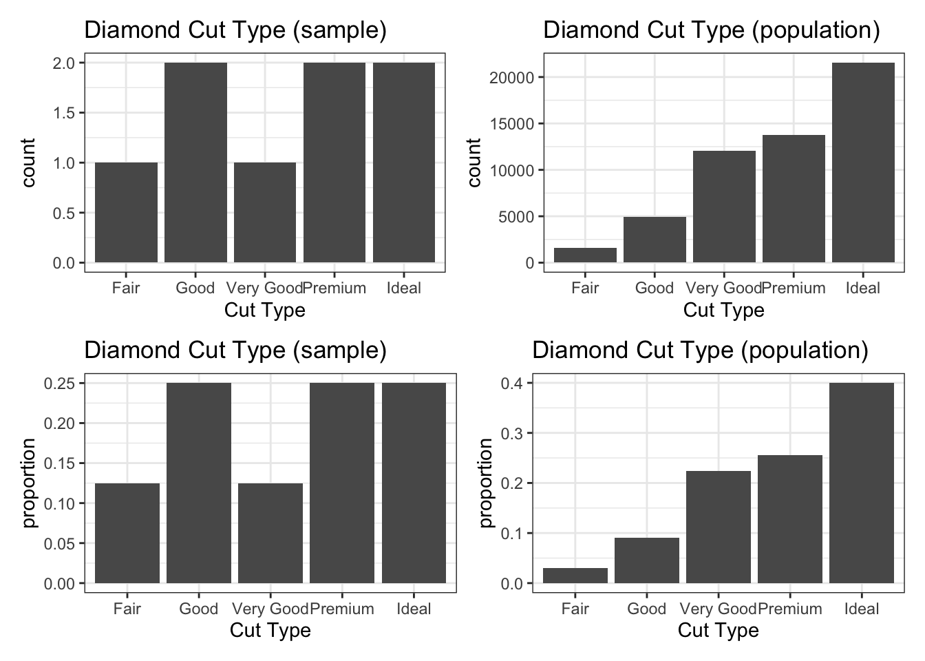
We’ll see how to create plots like these in the next notebook.

Submit

If you are part of a course with an instructor who is grading your work on these activities, please copy and submit both of the hashes below using the method your instructor has requested.

Question Hash

The hash below encodes your responses to the multiple choice and checkbox questions in this activity.

function getItem(key, fallback) {
  const val = localStorage.getItem(key);
  return val !== null ? JSON.parse(val) : fallback;
}

function buildQuestionResults() {
  return {
    notebook: "Topic 3: Descriptive Statistics",
    type: "questions",
    timestamp: new Date().toISOString(),
    questions: {
      q1_measures_of_center: {
        selected: getItem("q1_selected", null),
        correct_answer: "4",
        result: localStorage.getItem("q1_result") ?? "unattempted"
      },
      q2_sampling_validity_1: {
        selected: getItem("q2_selected", null),
        correct_answer: "3",
        result: localStorage.getItem("q2_result") ?? "unattempted"
      },
      q3_sampling_validity_2: {
        selected: getItem("q3_selected", []),
        correct_answer: "1,2,5",
        result: localStorage.getItem("q3_result") ?? "unattempted"
      },
      q4_measures_of_center_2: {
        selected: getItem("q4_selected", []),
        correct_answer: "1,3",
        result: localStorage.getItem("q4_result") ?? "unattempted"
      },
      q5_measures_of_spread_1: {
        selected: getItem("q5_selected", null),
        correct_answer: "3",
        result: localStorage.getItem("q5_result") ?? "unattempted"
      },
      q6_measures_of_spread_2: {
        selected: getItem("q6_selected", null),
        correct_answer: "1",
        result: localStorage.getItem("q6_result") ?? "unattempted"
      }
    }
  };
}

function toBase64(str) {
  return btoa(unescape(encodeURIComponent(str)));
}

question_hash = {
  q1; q2; q3; q4; q5; q6;
  
  const results = {
    notebook: "Topic 3: Descriptive Statistics",
    type: "questions",
    timestamp: new Date().toISOString(),
    questions: {
      q1_measures_of_center: {
        selected: q1,
        correct_answer: "4",
        result: q1 === null ? "unattempted" : (q1 == 4 ? "correct" : "incorrect")
      },
      q2_sampling_validity_1: {
        selected: q2,
        correct_answer: "3",
        result: q2 === null ? "unattempted" : (q2 == 3 ? "correct" : "incorrect")
      },
      q3_sampling_validity_2: {
        selected: q3 ?? [],
        correct_answer: "1,2,5",
        result: (!q3 || q3.length === 0) ? "unattempted" : (q3.toString() === "1,2,5" ? "correct" : "incorrect")
      },
      q4_measures_of_center_2: {
        selected: q4 ?? [],
        correct_answer: "1,3",
        result: (!q4 || q4.length === 0) ? "unattempted" : (q4.toString() === "1,3" ? "correct" : "incorrect")
      },
      q5_measures_of_spread_1: {
        selected: q5,
        correct_answer: "3",
        result: q5 === null ? "unattempted" : (q5 == 3 ? "correct" : "incorrect")
      },
      q6_measures_of_spread_2: {
        selected: q6,
        correct_answer: "1",
        result: q6 === null ? "unattempted" : (q6 == 1 ? "correct" : "incorrect")
      }
    }
  };
  
  return toBase64(JSON.stringify(results));
}

html`<div style="font-family: monospace; font-size: 0.85em; background: #f5f5f5; padding: 12px; border-radius: 6px; word-break: break-all; border: 1px solid #ddd; user-select: all; cursor: pointer;" onclick="navigator.clipboard.writeText(this.innerText)">
  ${question_hash}
</div>
<p style="margin-top: 8px; font-size: 0.9em; color: #555;">
  Click the box to copy to clipboard.
</p>`

Exercise Hash

Click the button below to generate your exercise submission code. This hash encodes your work on the graded code exercises in this activity.

You must have attempted the graded exercises before clicking — clicking generates a snapshot of your current results. If you have completed the activity over multiple sessions, please go back through and hit the Run Code button on each graded exercise before generating the hash below, to ensure your most recent results are recorded.

Summary

Main Takeaways

• We can summarize numerical data using measures of central tendency and measures of spread (or variability).
• The mean (\(\bar{x}\) for samples, \(\mu\) for populations) and median measure the center of a set of numerical data.
• The standard deviation (\(s\) for samples, \(\sigma\) for populations) and interquartile range (\(IQR\)) measure the spread of a set of numerical data.
• The median and \(IQR\) are robust measures in the presence of outliers (unusually large or small values) — the mean and standard deviation are not.
• Categorical data is best summarized in a frequency table or relative frequency table.

R Commands Introduced

• Compute the mean:

data_frame_name |>
  summarize(avg_column_name = mean(column_name))
# or
mean(data_frame_name$column_name)

• Compute the median:

data_frame_name |>
  summarize(median_column_name = median(column_name))
# or
median(data_frame_name$column_name)

• Compute the standard deviation:

data_frame_name |>
  summarize(sd_column_name = sd(column_name))
# or
sd(data_frame_name$column_name)

• Compute the boundaries for the interquartile range:

data_frame_name |>
  summarize(quantile_column_name = quantile(column_name, probs = c(0.25, 0.75)))
# or
quantile(data_frame_name$column_name, probs = c(0.25, 0.75))

• Compute the interquartile range:

data_frame_name |>
  summarize(IQR_column_name = IQR(column_name))
# or
IQR(data_frame_name$column_name)

• Compute general percentiles:

data_frame_name |>
  summarize(percentile_column_name = quantile(column_name, probs = c(p1, p2, ...)))
# or
quantile(data_frame_name$column_name, probs = c(p1, p2, ...))

• Build a frequency table:

data_frame_name |>
  count(column_name)
# or
table(data_frame_name$column_name)

• Build a relative frequency table:

data_frame_name |>
  count(column_name) |>
  mutate(relative_frequency = n / sum(n))
# or
table(data_frame_name$column_name) / nrow(data_frame_name)

Looking Ahead

In the next activity we’ll shift from summarizing data numerically to visualizing it. We’ll learn how to construct histograms, boxplots, and bar charts in R using ggplot2. In addition to syntax and structure, you’ll develop intuition for choosing the right visualization for a given variable type(s) and question.

References

[1] Wickham, H. (2016). ggplot2: Elegant graphics for data analysis [Diamonds Dataset]. Springer-Verlag New York. https://ggplot2.tidyverse.org/