Topic 1: An Introduction to Data and Sampling

function ok_checkbox(response, n) {
  if (!response || response.length === 0) 
    return html`<span style="color:purple">You haven't answered yet.</span>`;
  if (response.toString() === n) 
    return html`<span style="color:green">Correct ✓</span>`;
  return html`<span style="color:red">Not Yet! ✗</span>`;
}

About

This activity covers an introduction to data, variable types (numeric and categorical variables, along with unique identifiers), and strategies for data collection.

{
  const btn = html`<button style="
    background: #436b95;
    color: white;
    border: none;
    padding: 8px 16px;
    border-radius: 4px;
    cursor: pointer;
    font-size: 0.9em;
  ">🔄 Reset My Responses</button>`;

  btn.onclick = () => {
    if (confirm('Reset all responses for this activity? This cannot be undone.')) {
      Object.keys(localStorage)
        .filter(k => k.endsWith('_selected_t1') || k.endsWith('_correct_t1') || k.endsWith('_result_t1'))
        .forEach(k => localStorage.removeItem(k));
      location.reload();
    }
  };

  return btn;
}

Data and Sampling

This is the first of a series of interactive workbooks you’ll use to engage with content from introductory statistics. This workbook covers an introduction to data, including some limited background on experimental design and data collection.

An Introduction to Data

In this workbook you’ll encounter two datasets – one concerning real estate from King County, WA (houses) and another containing prices and attributes of almost 54,000 diamonds (diamonds). A few rows of the houses data are being shown below in a convenient form where the rows of data represent records (sometimes called observations), and the columns represent variables (sometimes called features). Data in this form is sometimes referred to as tidy.

id	month	price	sqft_living	sqft_lot	waterfront	exterior
7129300520	9	221900	1180	5650	0	shingles
6414100192	4	538000	2570	7242	0	vinyl siding
5631500400	12	180000	770	10000	0	brick
2487200875	12	604000	1960	5000	0	vinyl siding
1954400510	2	510000	1680	8080	0	shingles
7237550310	1	1225000	5420	101930	0	vinyl siding
1321400060	5	257500	1715	6819	0	brick
2008000270	3	291850	1060	9711	0	vinyl siding
2414600126	2	229500	1780	7470	0	shingles
3793500160	6	323000	1890	6560	0	vinyl siding

You can see the first six rows of the houses dataset above. A limited data dictionary (a map of column names and explanations) appears below.

• id provides the property identification number.
• month gives the month that the property was listed for sale.
• price is the listing price of the property in US dollars ($).
• sqft_living gives the finished square footage of the home.
• sqft_lot gives the square footage of the property (land).
• waterfront indicates whether the property is waterfront.
• exterior provides a description of the exterior covering of the home.

Variable Types

We’ll encounter different types of variables/data in our course. Knowing the type of a variable is critical because the data type often dictates how we can utilize/summarize that variable.

• Variables which take on numerical values and for which measures such as the mean, median, or standard deviation are meaningful are referred to as numerical.

• Variables which serve to group data into categories are called categorical.

  • Examples include the color of a car or an area code prefix for a telephone number.
  • Note that a telephone area code looks numeric, but since taking their average is meaningless, we consider it to be categorical.

• A unique identifier is a variable which is neither numerical, nor does it have any grouping value.

  • A student ID number is an example of a unique identifier.
  • However, with a bit of pre-processing we can sometimes extract useful information from these types of variables. The strategies for doing so will be outside the scope of our course.

Answer the following using your knowledge of the dataset and variable types.

Check Your Understanding: Numerical Variables

Check off each of the variables from the houses data set which are numerical.

mutable ok_response = (response, n) => { return html`Loading...` };
viewof q1 = Inputs.checkbox(
  new Map([
    ["id", 1],
    ["month", 2],
    ["price", 3],
    ["sqft_living", 4],
    ["sqft_lot", 5],
    ["waterfront", 6],
    ["exterior", 7]
  ]),
  {value: JSON.parse(localStorage.getItem("q1_selected_t1") ?? "[]") ?? []}
);

{
  localStorage.setItem("q1_selected_t1", JSON.stringify(q1));
  localStorage.setItem("q1_correct_t1", "3,4,5");
  localStorage.setItem("q1_result_t1", (!q1 || q1.length === 0) ? "unattempted" : (q1.toString() === "3,4,5" ? "correct" : "incorrect"));
}

ok_checkbox(q1, "3,4,5");

Check Your Understanding: Categorical Variables

Check off each of the variables from the houses dataset which are categorical.

viewof q2 = Inputs.checkbox(
  new Map([
    ["id", 1],
    ["month", 2],
    ["price", 3],
    ["sqft_living", 4],
    ["sqft_lot", 5],
    ["waterfront", 6],
    ["exterior", 7]
  ]),
  {value: JSON.parse(localStorage.getItem("q2_selected_t1") ?? "[]") ?? []}
);

{
  localStorage.setItem("q2_selected_t1", JSON.stringify(q2));
  localStorage.setItem("q2_correct_t1", "2,6,7");
  localStorage.setItem("q2_result_t1", (!q2 || q2.length === 0) ? "unattempted" : (q2.toString() === "2,6,7" ? "correct" : "incorrect"));
}

ok_checkbox(q2, "2,6,7");

Check Your Understanding: Unique Identifiers

Check off each of the variables from the houses dataset which are unique identifiers.

viewof q3 = Inputs.checkbox(
  new Map([
    ["id", 1],
    ["month", 2],
    ["price", 3],
    ["sqft_living", 4],
    ["sqft_lot", 5],
    ["waterfront", 6],
    ["exterior", 7]
  ]),
  {value: JSON.parse(localStorage.getItem("q3_selected_t1") ?? "[]") ?? []}
);

{
  localStorage.setItem("q3_selected_t1", JSON.stringify(q3));
  localStorage.setItem("q3_correct_t1", "1");
  localStorage.setItem("q3_result_t1", (!q3 || q3.length === 0) ? "unattempted" : (q3.toString() === "1" ? "correct" : "incorrect"));
}

ok_checkbox(q3, "1");

The levels of a variable are the different (distinct) values that the variable takes on. For example, a dataset on students might include a variable called ClassYear with the levels Freshman, Sophomore, Junior, Senior. Numerical variables also have levels – usually there are lots of levels corresponding to a numerical variable, but if there are too few, we may be better off considering the corresponding variable to be categorical. For example, if we had a dataset that included a Year variable, but its only observed levels in the dataset are 2008 and 2017, we may be better off thinking about Year as a categorical variable than as a numerical one.

Tip

If a numerical variable has very few levels, you may be better off treating it as a categorical variable.

Relationships between variables

Association, Independence, Correlation: Two variables are associated with one another if a change in levels of one is generally accompanied by change in the other. This may be that larger values of one variable are accompanied by larger (or smaller) values in the other. Think – “does knowing something about one of the variables give me any information about the other?” If two variables are not associated, then we might say that they are independent of one another. Lastly, correlation is a way to formally measure the strength of a LINEAR association between two variables. Look at the plots considering characteristics of various diamonds below.

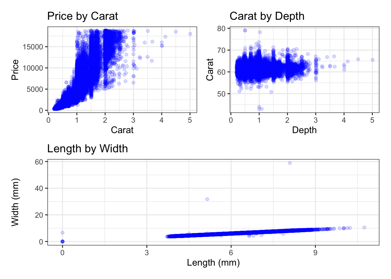
Use the plots above to answer the following questions.

Check Your Understanding: Associations

Which of the plots above highlight an association between the corresponding variables?

viewof q4 = Inputs.checkbox(
  new Map([
    ["Carat versus Price", 1],
    ["Depth versus Carat", 2],
    ["Length by Width", 3]
  ]),
  {value: JSON.parse(localStorage.getItem("q4_selected_t1") ?? "[]") ?? []}
);

{
  localStorage.setItem("q4_selected_t1", JSON.stringify(q4));
  localStorage.setItem("q4_correct_t1", "1,3");
  localStorage.setItem("q4_result_t1", (!q4 || q4.length === 0) ? "unattempted" : (q4.toString() === "1,3" ? "correct" : "incorrect"));
}

ok_checkbox(q4, "1,3");

Check Your Understanding: Independence

Which pair of variables from the above plots is independent?

viewof q5 = Inputs.radio(
  new Map([
    ["Carat versus Price", 1],
    ["Depth versus Carat", 2],
    ["Length by Width", 3]
  ]),
  {value: JSON.parse(localStorage.getItem("q5_selected_t1") ?? "null")}
);

{
  localStorage.setItem("q5_selected_t1", JSON.stringify(q5));
  localStorage.setItem("q5_correct_t1", "2");
  localStorage.setItem("q5_result_t1", q5 === null ? "unattempted" : (q5 == 2 ? "correct" : "incorrect"));
}

ok_response(q5, "2");

Check Your Understanding: Correlation

Which of the plots shows the strongest correlation between the corresponding variables?

viewof q6 = Inputs.radio(
  new Map([
    ["Carat versus Price", 1],
    ["Depth versus Carat", 2],
    ["Length by Width", 3]
  ]),
  {value: JSON.parse(localStorage.getItem("q6_selected_t1") ?? "null")}
);

{
  localStorage.setItem("q6_selected_t1", JSON.stringify(q6));
  localStorage.setItem("q6_correct_t1", "3");
  localStorage.setItem("q6_result_t1", q6 === null ? "unattempted" : (q6 == 3 ? "correct" : "incorrect"));
}

ok_response(q6, "3");

Directionality of Associations

Since both of the variables in each of the plots above are numerical, we can describe the direction of the association.

• Two variables are said to be positively associated if an increase in the observed level of one variable is generally accompanied by an increase in the level of the other.

  • Notice that there is a positive association in both of the plots you identified above

• Two variables are said to be negatively associated if an increase in the level of one is generally accompanied by a decrease in the other

• It is also possible for variables to exhibit non-linear associations with one another.

We can also identify whether an association exists between variables when one or more are categorical. Remember, you’re asking “does knowing something about the observed level of one of the variables tell me anything about the other?” Consider the plots below which refer back to our houses dataset from earlier.

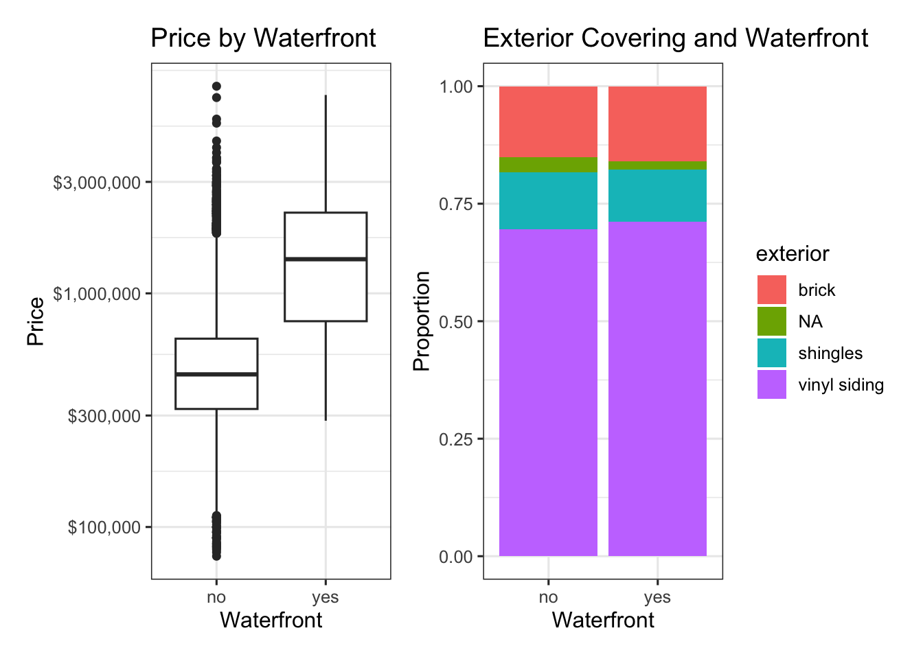
Check Your Understanding: Associations II

One of the plots above shows a clear association between the corresponding variables. Which one is it?

viewof q7 = Inputs.radio(
  new Map([
    ["Price by Waterfront Status", 1],
    ["Exterior Covering and Waterfront Status", 2]
  ]),
  {value: JSON.parse(localStorage.getItem("q7_selected_t1") ?? "null")}
);

{
  localStorage.setItem("q7_selected_t1", JSON.stringify(q7));
  localStorage.setItem("q7_correct_t1", "1");
  localStorage.setItem("q7_result_t1", q7 === null ? "unattempted" : (q7 == 1 ? "correct" : "incorrect"));
}

ok_response(q7, "1");

Check your answer against the correct response. What makes that answer the best choice? If you’re unsure, ask a question to a friend, mentor, or teacher and work it out together.

Major Questions In Statistics

Given groups with different characteristics (differing levels) regarding variable X, do they differ with respect to variable Y?

For example, we might ask is the average listing price of a waterfront home greater than the average listing price of a home which is not on the waterfront in King County, WA. In this example, X is whether or not the home is on the waterfront and Y is the listing price of the home.

We’ll find that we can’t just answer these questions by looking at plots involving some sample data. Why not?

Data collection principles

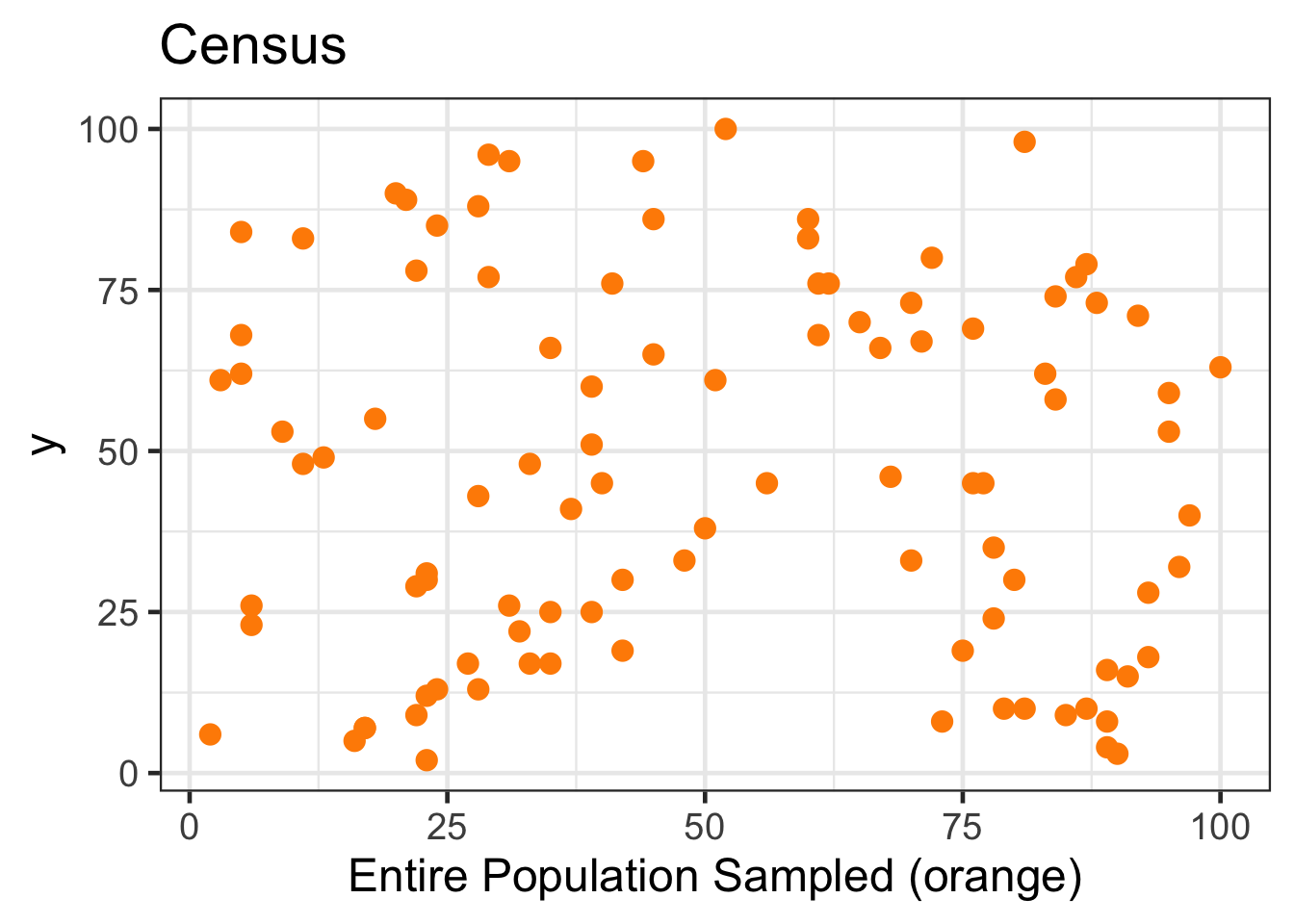
Population versus Sample: In statistics, we almost always want to apply generalizations from a small sample to a large population – you might think of this as a sort of stereotyping. The trick here is that for our assertions (generalizations) to be valid, our sample must be representative of our population.

Critical Takeaway

Results based off of a sample may only be generalized to a population for which that sample is representative.

Sampling Strategies: There are many sampling techniques. We will focus on census, simple random sample, stratified sample, and convenience sample.

If we could sample every object in a population we would be taking a census. While census would give us certainty in an answer to a statistical question, it is not feasible to conduct a census due to phenomenon such as non-response and fluid populations.

Please Listen to this NPR story which aired prior to the 2010 Census

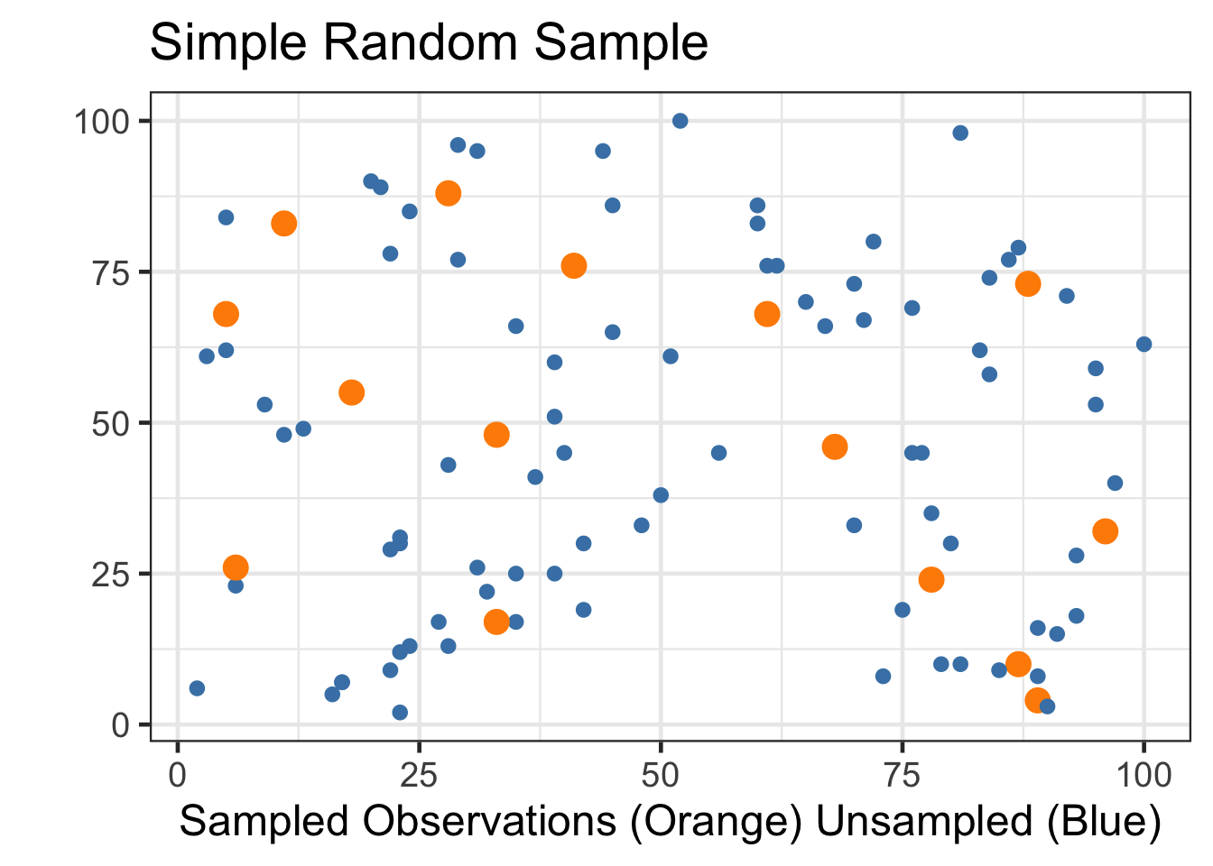
The simple random sample is the GOLD STANDARD in statistics. We randomly select some “large enough” number of individual items from the entire population and take measurements on our variables of interest. The advantage of the simple random sample is that we are likely to attain a sample of results that are representative of the entire population.

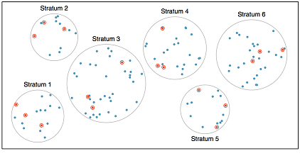
The stratified sample is used to ensure that we include representatives of all groups within our sample. Stratified sampling is particularly useful in cases where the population is segmented (that is, there are clear groups which may potentially have different responses)

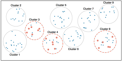
The cluster sample is used when we can argue that there are many small “populations” that are truly representative of the larger population. The clustering method is typically used to reduce costs (financial or otherwise). From the collection of clusters, a random sample is selected and as many observations as possible are collected from within each of those chosen clusters.

A variation on clustering is called two-stage or multi-stage sampling. With this method, observations are first clustered and clusters are chosen at random. Second, within each of the chosen clusters a simple random sample is taken. Notice that this method occurs in two stages, as the name suggests.

The convenience sample is the most commonly used sampling method. Unfortunately, it is also the worst. When researchers sample from individuals they have “easy access” to, they are conducting a convenience sample. There are always hidden biases in these samples. Here’s a famous example in which the Literary Digest incorrectly predicted a landslide victory for Alf Landon over FDR in the 1936 US Presidential Election. In addition, much of the error in predicting the results of the 2016 presidential election may be attributable to convenience sampling.

Experimental Design

Experiment versus Observational Study: Beyond just sampling, there are multiple methods for collecting data. We can just observe what happens naturally (without manipulating any conditions) or we can run an experiment. In experiments we manipulate one or more conditions, utilizing a control and treatment group(s). The advantage to an experiment is that we can infer cause and effect relationships (this is extremely important in medical studies), but in observational studies we can only discuss an association between variables.

Explanatory versus Response Variables: Typically in statistics we will identify a question (a claim about a response variable) with respect to a population. We will take a representative sample of that population and collect observed responses as well as observations on other variables (perhaps age, level of formal education, political affiliation, etc). These additional variables are called explanatory variables. In general, explanatory variables are variables which we expect may be associated with the response variable.

There’s lots more to learn about experimental design, but it is beyond the scope of this notebook. You should read pages 32 through 35 of OpenIntro Statistics, 4Ed as a starting point.

Submit

If you are part of a course with an instructor who is grading your work on these activities, please copy and submit both of the hashes below using the method your instructor has requested (there is only a question hash for this activity, no exercise hash).

Question Hash

The hash below encodes your responses to the multiple choice and checkbox questions in this activity.

function buildQuestionResults() {
  return {
    notebook: "Topic 1: An Introduction to Data and Sampling",
    type: "questions",
    timestamp: new Date().toISOString(),
    questions: {
      q1_numerical_variables: {
        selected: q1,
        correct_answer: "3,4,5",
        result: (!q1 || q1.length === 0) ? "unattempted" : (q1.toString() === "3,4,5" ? "correct" : "incorrect")
      },
      q2_categorical_variables: {
        selected: q2,
        correct_answer: "2,6,7",
        result: (!q2 || q2.length === 0) ? "unattempted" : (q2.toString() === "2,6,7" ? "correct" : "incorrect")
      },
      q3_unique_identifiers: {
        selected: q3,
        correct_answer: "1",
        result: (!q3 || q3.length === 0) ? "unattempted" : (q3.toString() === "1" ? "correct" : "incorrect")
      },
      q4_associations: {
        selected: q4,
        correct_answer: "1,3",
        result: (!q4 || q4.length === 0) ? "unattempted" : (q4.toString() === "1,3" ? "correct" : "incorrect")
      },
      q5_independence: {
        selected: q5,
        correct_answer: "2",
        result: q5 === null ? "unattempted" : (q5 == 2 ? "correct" : "incorrect")
      },
      q6_correlation: {
        selected: q6,
        correct_answer: "3",
        result: q6 === null ? "unattempted" : (q6 == 3 ? "correct" : "incorrect")
      },
      q7_associations_2: {
        selected: q7,
        correct_answer: "1",
        result: q7 === null ? "unattempted" : (q7 == 1 ? "correct" : "incorrect")
      }
    }
  };
}

function toBase64(str) {
  return btoa(unescape(encodeURIComponent(str)));
}

question_hash = {
  q1; q2; q3; q4; q5; q6; q7;
  return toBase64(JSON.stringify(buildQuestionResults()));
}

html`<div style="font-family: monospace; font-size: 0.85em; background: #f5f5f5; padding: 12px; border-radius: 6px; word-break: break-all; border: 1px solid #ddd; user-select: all; cursor: pointer;" onclick="navigator.clipboard.writeText(this.innerText)">
  ${question_hash}
</div>
<p style="margin-top: 8px; font-size: 0.9em; color: #555;">
  Click the box to copy to clipboard.
</p>`

Exercise Hash

Since there were no code cell exercises in this activity, there is no exercise hash to generate. You’ll see exercise hashes in future activities.

Summary

Main Takeaways

• Data is stored in a table called a data frame. The rows of the data frame are observations and the columns are collected variables.
• Within this introductory course, data is either numerical, categorical, or unique identifier — to determine type, ask “is the average of these observations meaningful?” and “does this variable provide grouping value?”
• Two variables are associated if a change in one has some (even limited) predictive value about a change in the other. If no such relationship exists, the variables are independent.
• Correlation formally measures the strength of a linear association between two numerical variables.
• There are many ways data can be collected, but in order to produce meaningful results we must use random sampling.
• Results from a sample can be generalized only to a population for which that sample is representative.

Looking Ahead

The next activity introduces R — the statistical computing environment we’ll use throughout this course. You’ll learn how to use R as a calculator and get your first exposure to working with data frames. The diamonds dataset you met here will make a return appearance.

References

[1] House Sales in King County, USA (2016). Kaggle. Retrieved from Kaggle House Sales Dataset.
[2] Wickham, H. (2016). ggplot2: Elegant graphics for data analysis [Diamonds Dataset]. Springer-Verlag New York. https://ggplot2.tidyverse.org/