MAT 370: Polynomial Interpolation
December 29, 2025
Interpolation and Curve-Fitting
Through this next section of our course, we’ll consider fitting models to observed data.
There are two umbrella processes for achieving this objective – interpolation or curve fitting.
Interpolation assumes a deterministic relationship with observed data assumed to be measured exactly.
Curve-fitting is a process that acknowledges noise and uncertainty and seeks to capture a general trend between available independent features and a dependent response.

Polynomial Interpolation
We’ve seen that interpolation means fitting curves through existing data points.
That is, our observed data points will fall exactly on the curve(s) we are constructing.
It is always possible to construct a unique polynomial of degree at most \(n-1\) that passes through \(n\) distinct data points having distinct “\(x\)” coordinates.
A Strategy and an Example
As usual, we’ll find it helpful to have an example to work with while we introduce and discuss the methods for polynomial interpolation below.
\[P_{n}\left(x\right) = \sum_{i = 0}^{n}{y_i\ell_{i}\left(x\right)}\]
where \(n\) is the degree of the polynomial and
\[\begin{align*} \ell_{i}\left(x\right) &= \left(\frac{x - x_0}{x_i - x_0}\right)\left(\frac{x - x_1}{x_i - x_1}\right)\cdots \left(\frac{x - x_{i-1}}{x_i - x_{i-1}}\right)\left(\frac{x - x_{i+1}}{x_i - x_{i+1}}\right)\cdots \left(\frac{x - x_n}{x_i - x_n}\right)\\ &= \prod_{\substack{j=0\\ j\neq i}}^{n}{\frac{x - x_{j}}{x_i - x_j}}~~\text{for}~~i = 0, 1, \cdots, n \end{align*}\]
The \(\ell_{i}\left(x\right)\) functions are called the cardinal functions.
Note that if \(n = 1\) (two points), we have a linear function:
\[P_1\left(x\right) = y_0\left(\frac{x - x_1}{x_0 - x_1}\right) + y_1\left(\frac{x - x_0}{x_1 - x_0}\right)\]
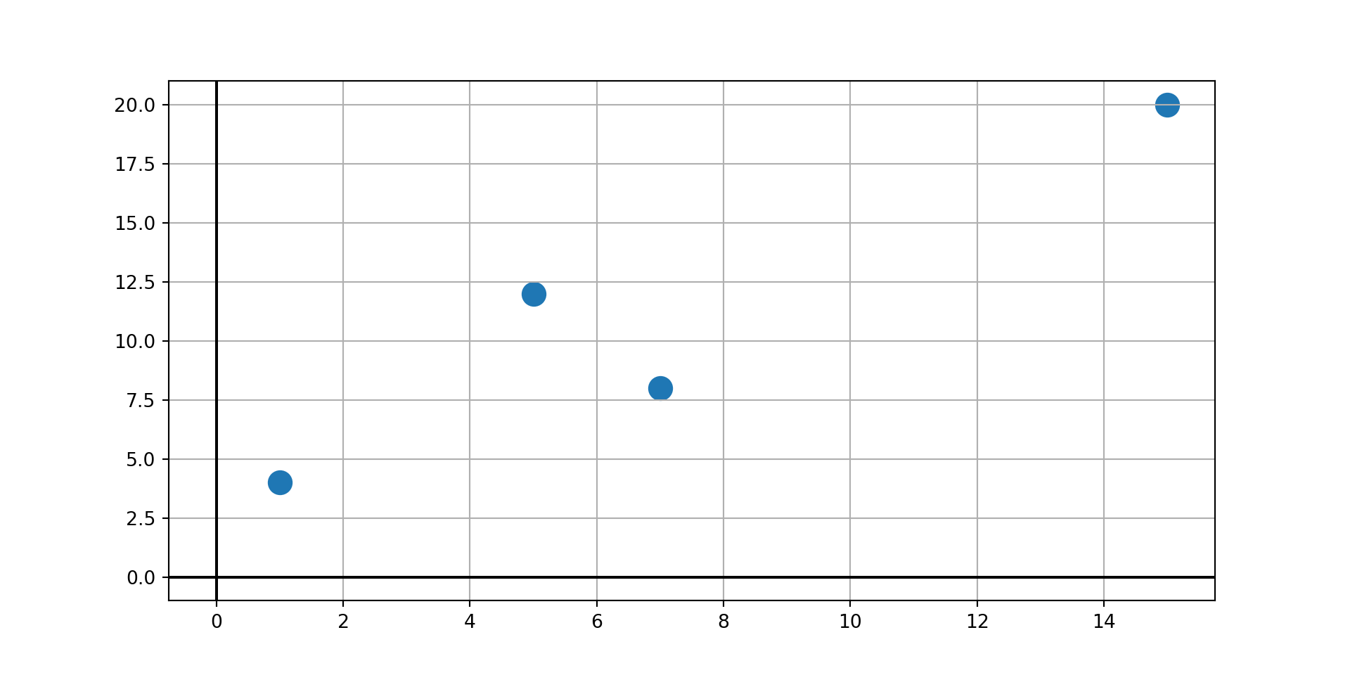
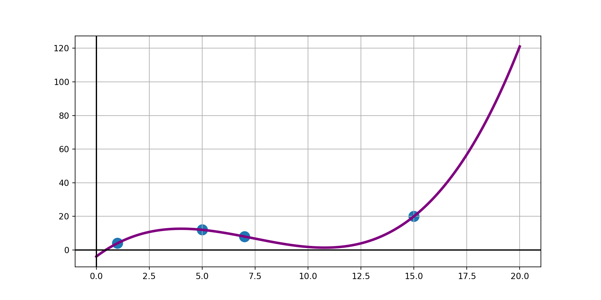
Example: Construct a degree-three polynomial interpolant for the observed data
| x | y |
|---|---|
| 1 | 4 |
| 5 | 12 |
| 7 | 8 |
| 15 | 20 |
Completing the Example
Example: Use Lagrange’s Method to find a third degree polynomial interpolant through the observed data points \(\left(1, 4\right)\), \(\left(5, 12\right)\), \(\left(7, 8\right)\), and \(\left(15, 20\right)\).
As a reminder, the Lagrange polynomial consists of sums of terms of the form
\[y_i\prod_{\substack{j = 0\\ j\neq i}}^{n}\left(\frac{x - x_i}{x_i - x_j}\right)\]
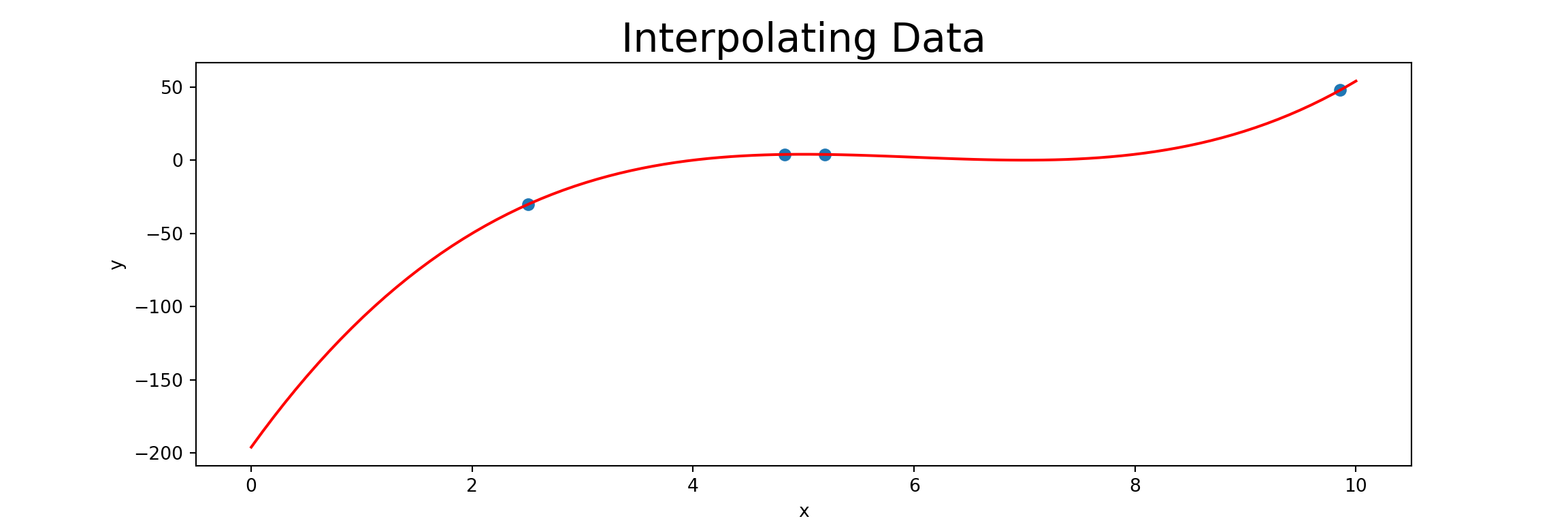
Using the Newton’s Method Algorithm
xData = np.random.uniform(0, 10, 4)
yData = np.random.uniform(0, 10, 4)

coefs = getCoefficients(xData, yData)

x_new = np.linspace(0, 10, 100)
y_new = evaluatePolynomial(coefs, xData, x_new)

plt.scatter(xData, yData, s = 150)
plt.plot(x_new, y_new, color = "purple", linewidth = 3)
plt.grid()
plt.axhline(color = "black")
plt.axvline(color = "black")
plt.ylim((-50, 50));
plt.xlabel("x")
plt.ylabel("y")
plt.title("Data and Interpolated Polynomial (Newton's Method)", fontsize = 22)
plt.show()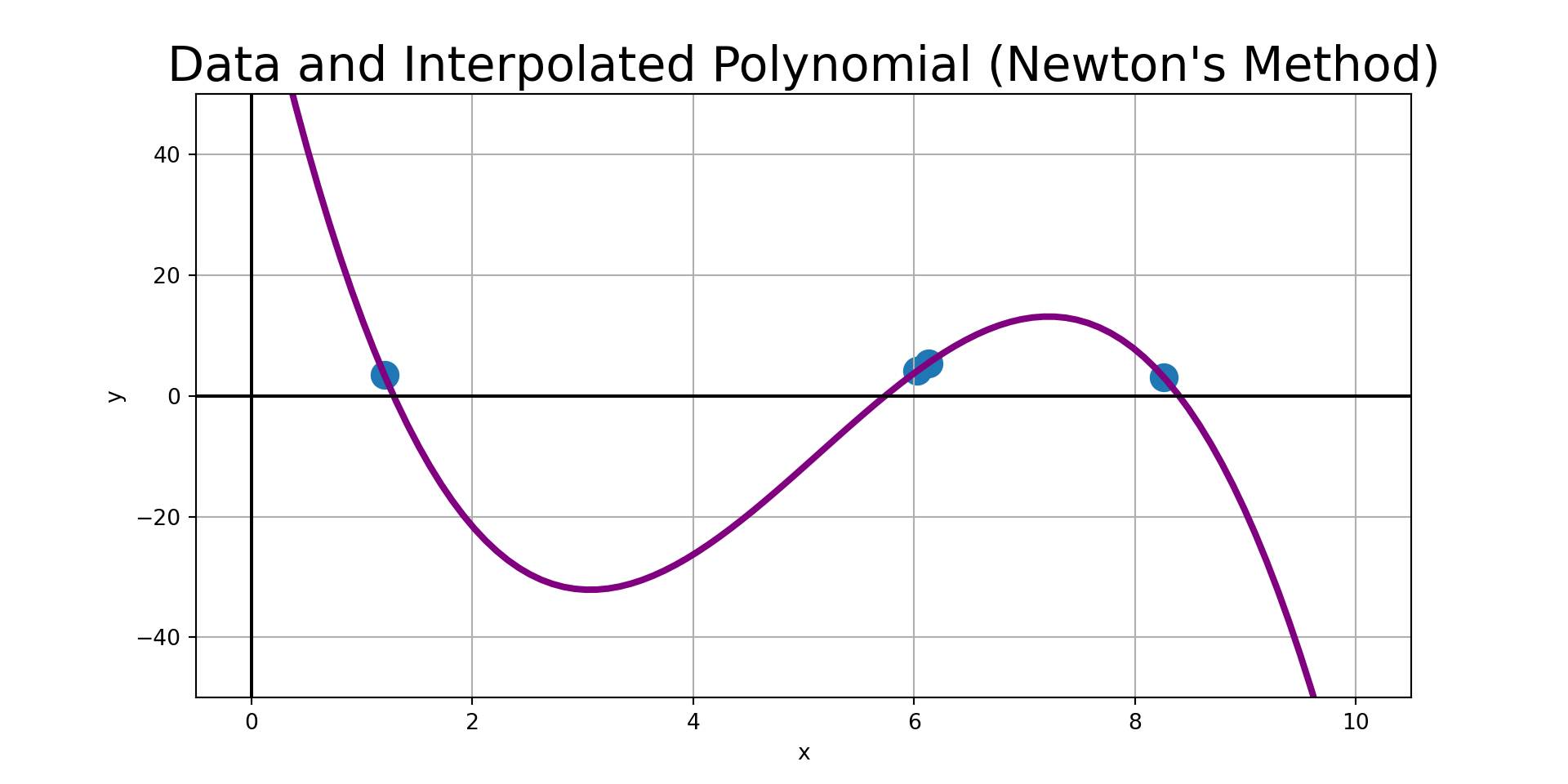
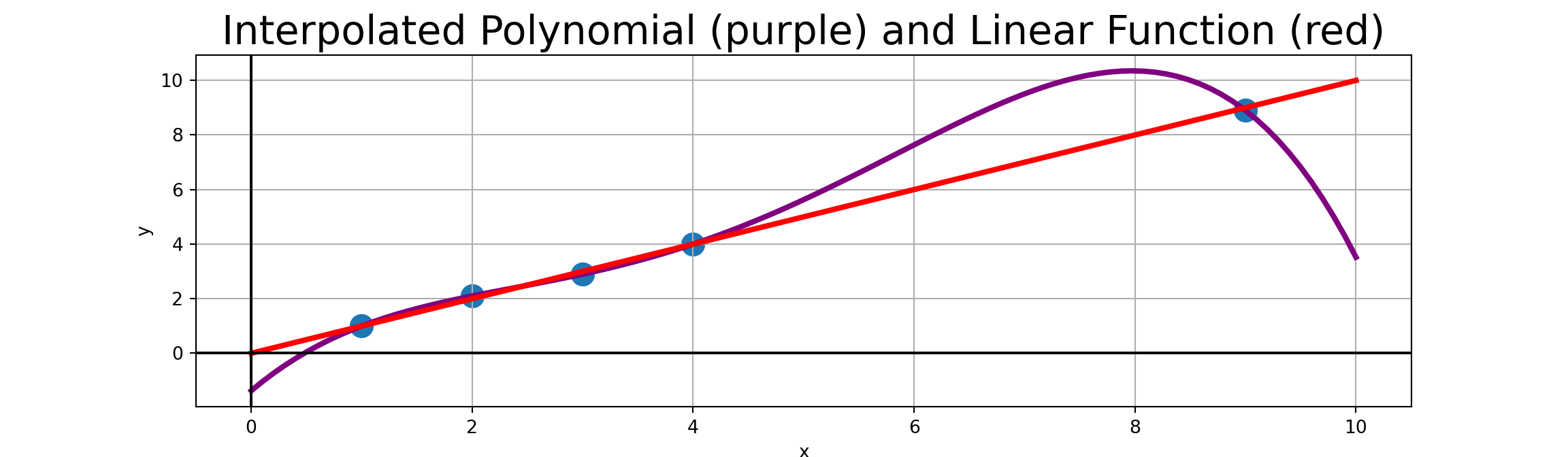
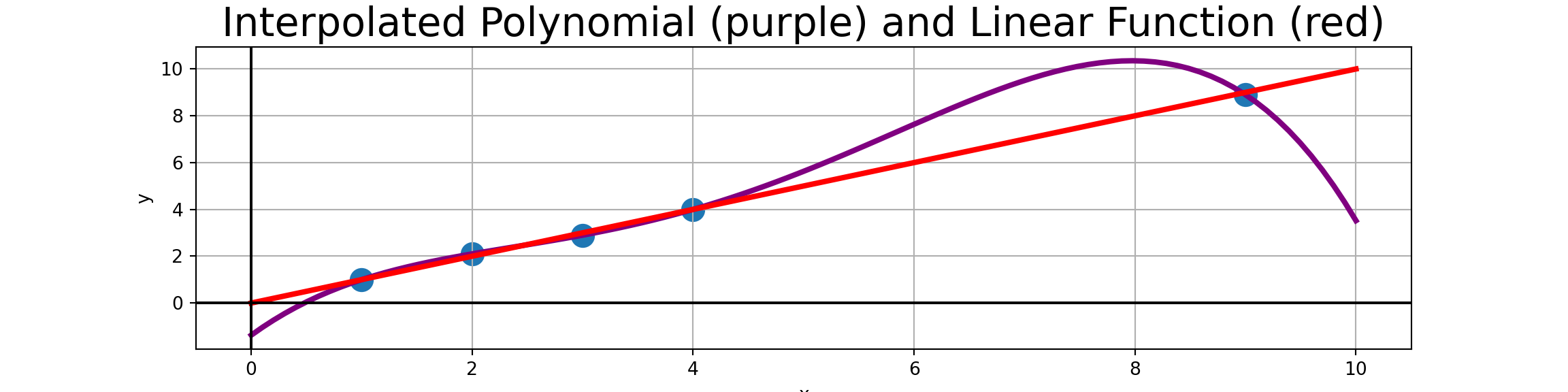
Limitations to Polynomial Interpolation
Including additional observed data points automatically increases the degree of the interpolated polynomial.
This can be really detrimental, especially if there is slight noise in the measured observations.
For example, consider the nearly-linear data points to the right.
| x | y |
|---|---|
| 1 | 1 |
| 2 | 2.1 |
| 3 | 2.9 |
| 4 | 4 |
| 9 | 8.9 |
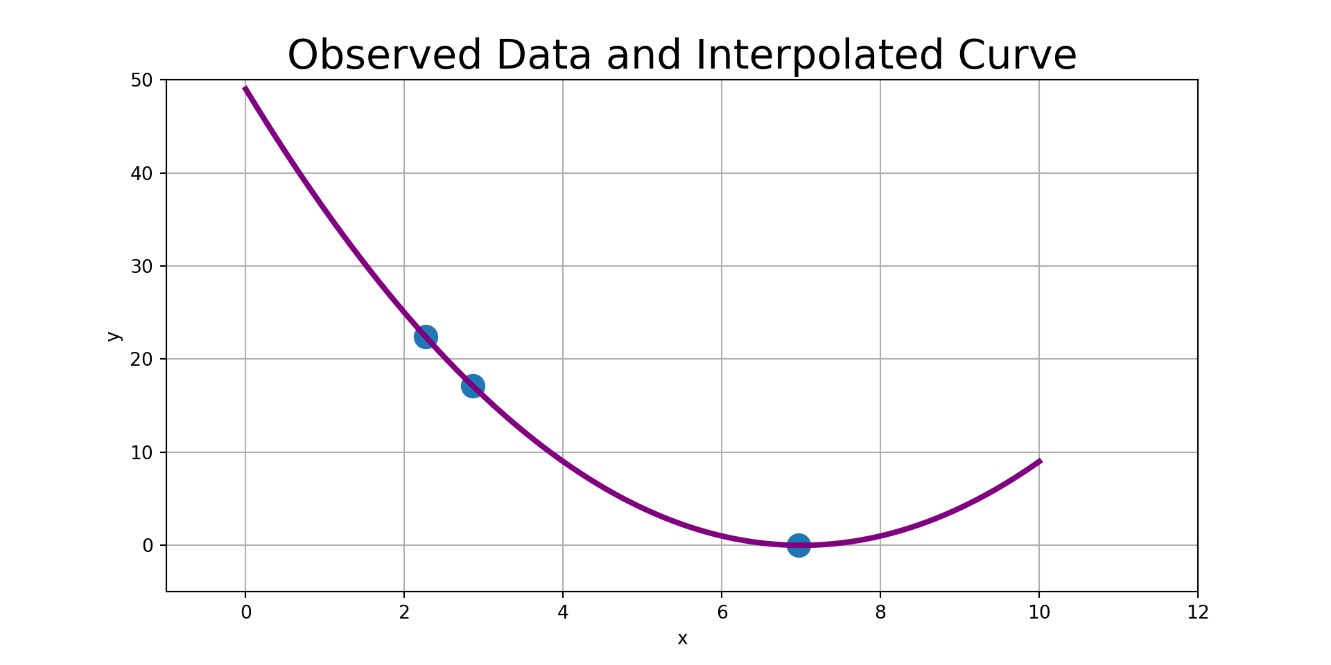
A Note on Extrapolation
Extrapolation means using a model to make predictions for values of the independent variable(s) beyond which we have support for.
An easy way to think of this is that these are values below the minimum observed value or above the maximum observed value (though these are not the only scenarios).
In cases where you must extrapolate, use a low-order (small degree) polynomial interpolated only on the nearest-neighbor observations.
Additionally, you should plot the interpolated polynomial for visual confirmation that the extrapolation makes sense.
For example, in the plot of the interpolated polynomial on the nearly-linear data earlier, we can clearly see that using that red polynomial to extrapolate \(p\left(10\right)\) is not a good idea.
Comments on Limitations
We can see that the interpolated polynomial has emphasized bends to accommodate the “measurement error”. Interpolated values for \(4 < x < 9\) should almost surely not be trusted.
General Rule 1: Polynomial extrapolation (interpolating outside the range of observed values) should be avoided.
General Rule 2: Polynomial interpolation should be carried out with the fewest number of data points feasible. For example, if you suspect that your polynomial should be degree \(2\), then use three data points. An interpolated polynomial passing through more than \(6\) observed data points should be viewed with extreme suspicion – In fact, the more data points used, the more suspicious we should be of our polynomial.