MAT 370: A Crash Course in Numerical Python

Dr. Gilbert

December 25, 2025

Reminders: Colab and Jupyter

So far we’ve been exposed to the following ideas about Jupyter Notebooks and Google Colab

• Google Colab provides an interface for writing Jupyter notebooks in your web browser via Google Drive

• Jupyter notebooks allow you to mix text (white background) and executable Python code (grey background) in a single document.

  • You execute code cells by holding down Shift and hitting Enter (or Return).

Reminders: Python So Far…

At our first class meeting, we got a broad overview of Python. We introduced the following ideas.

• We can use Python as a calculator, to carry out mathematical operations.
• We can store objects as variables to be reused later.
• We can use for and while loops to carry out the same sets of instructions over and over again.
• We can use conditional statements (if/else if/else) to control when certain instructions are to be run.
• We can (and should!) organize code into functions that can be applied and used in different contexts.

We also explored Python lists quite a bit and, while we won’t often explicitly use them, they’ll be part of how we define arrays (ie. vectors and matrices)

Setting Expectations

This notebook covers a crash course in numerical python and the numpy module.

After working through this notebook, you’ll have enough to get you started, but we’ll continue to learn more about python and numpy as the semester progresses.

\(\bigstar\) You will not, and should not expect to, be an expert or be fluent after today’s discussion. Expect to come back here and to our initial slide deck often. \(\bigstar\)

Today, we’ll revisit items in greater detail and visit some new ones as well. We’ll see…

• Extending Python functionality by importing modules – specifically {numpy}
• Defining vectors and matrices using np.array()
• Looping operations
• Using print() statements
• Quickly initializing large arrays with specialized {numpy} functionality
• Creating, and working with, functions
• Plotting with {matplotlib}

Importing and Using Modules

• Base Python can do basic things like limited math, printing, etc.

• When users want to engage in specialized activities, they’ll import modules that extend Python’s functionality by running import module_name.

  • {numpy} (numerical python) is a module that supports arrays and mathematics on arrays – we’ll make use of this module often.
  • {matplotlib} is a plotting library that will also come in handy for us.

• Using functionality from a module requires namespacing – that is, we call numpy.function_name() to access and use a function from the {numpy} module.

  • To reduce typing, people will often alias their modules with the as keyword.
  • For example, import numpy as np is extremely common.

• Many modules are nested.

  • We can use np.linalg.det() to compute the determinant of a matrix.
  • We’ll often import matplotlib.pyplot as plt and then use plt.function_name() for plotting.

Working with {numpy}

The {numpy} module is one that we’ll make extensive use of this semester.

• In the majority of our work, we’ll be using scalars (single component, numerical values) and arrays.

  • A 1-D array is a vector.
  • A 2-D array is a matrix.

• In order to make use of arrays, we’ll need to extend Python’s functionality by importing the {numpy} module.

import numpy as np

• We can define arrays using np.array().
  • It is easiest to pass a list to np.array() to create an array, as we did in our first notebook.
  • To the right, we create three vectors and a matrix, storing each in their own variables.

myVec_v1 = np.array([1, -3, 8.5])
myVec_v2 = np.array([4, 5, 6])
myVec_v3 = np.array([10, -9. -4.5, 2, 6.3])

myMatrix_A = np.array([
  [1.1, 8, 3],
  [-2, 6, -11.4]
])

Arithmetic on Arrays

We can perform arithmetical operations on arrays as long as their dimensions are compatible.

Recall the contents of myVec_v1, myVec_v2, myVec_v3, and myMatrix_A.

print("v1 = ", myVec_v1, "\n",
      "v2 = ", myVec_v2, "\n",
      "v3 = ", myVec_v3, "\n",
      "A = ", myMatrix_A)

v1 =  [ 1.  -3.   8.5] 
 v2 =  [4 5 6] 
 v3 =  [ 10.  -13.5   2.    6.3] 
 A =  [[  1.1   8.    3. ]
 [ -2.    6.  -11.4]]

We’ll try executing arithmetic operations on these vectors and matrix below.

print(myVec_v1 + myVec_v2)

[ 5.   2.  14.5]

print(myVec_v1 - myVec_v3)

ValueError: operands could not be broadcast together with shapes (3,) (4,) 

print(myVec_v1 + myMatrix_A)

[[ 2.1  5.  11.5]
 [-1.   3.  -2.9]]

print(np.matmul(myMatrix_A, myVec_v1))

[   2.6 -116.9]

Do you notice anything surprising or questionable?

A Note on Error Messages

If you haven’t been playing along in a Colab/Jupyter notebook, please consider doing it.

You’ll notice that the error messages in these slides are abridged versions of what you’ll see in your notebook environment.

• In the notebooks, you’ll see a full error traceback.

  • Generally, I find the last line of the error printout to be the most informative.
  • After looking at that last line, I’ll scroll up to the top of the error printout where there is an indication of where the error was encountered in the code that I attempted to run.
  • There will be an arrow indicating the line of code causing the issue, and often a red squiggle in the actual code cell.

\(\bigstar\) Learn not to be afraid, intimidated, or frustrated by errors – with practice, you will get better at deciphering them. \(\bigstar\)

Float Versus Integer Arrays

We’ve already seen several examples of where Python might not behave in ways we would expect.

• We’ve experienced the pass by reference pitfall with lists.

• We’ve seen that Python will execute mathematically inappropriate expressions.

  • Adding a scalar to a vector increases each entry by that scalar.
  • Adding two arrays with incompatible sizes is sometimes executed without error or warning.

All of this means we must be diligent, compare our results to our expectations, and not blindly trust that Python has done what we expected.

I’ll try to highlight quirks that have bitten me in the past so that you don’t get caught by them. Inevitably, we’ll encounter new quirks as well.

Float Versus Integer Arrays

Importance of Explicitly Declaring Float Arrays: Python will sometimes try to save space by storing numbers using an integer data type, but integer arithmetic is not the same as float arithmetic.

We’ll define two matrices below.

myMatrix_B = np.array([
  [1, 2, 3],
  [4, 5, 6],
  [7, 8, 9],
  [10, 11, 12]
])

myMatrix_B

array([[ 1,  2,  3],
       [ 4,  5,  6],
       [ 7,  8,  9],
       [10, 11, 12]])

myMatrix_C = np.array([
  [1.0, 2, 3],
  [4, 5, 6],
  [7, 8, 9],
  [10, 11, 12]
])

myMatrix_C

array([[ 1.,  2.,  3.],
       [ 4.,  5.,  6.],
       [ 7.,  8.,  9.],
       [10., 11., 12.]])

Can you tell that they are not treated the same by Python?

Defining Special Matrices

Sometimes we need to create somewhat large arrays, and typing in their entries one-by-one is not convenient or desirable.

We can construct an array of the appropriate size and then edit its contents via loops or accessing individual indices.

Each of the following are examples of methods that can be used to quickly construct arrays of a desired size.

my_2x5_zeros = np.zeros((2, 5))
my_2x5_zeros

my_4x4_id = np.identity(4)
my_4x4_id

my_dimC_ones = np.ones_like(myMatrix_C)
my_dimC_ones

array([[0., 0., 0., 0., 0.],
       [0., 0., 0., 0., 0.]])

array([[1., 0., 0., 0.],
       [0., 1., 0., 0.],
       [0., 0., 1., 0.],
       [0., 0., 0., 1.]])

array([[1., 1., 1.],
       [1., 1., 1.],
       [1., 1., 1.],
       [1., 1., 1.]])

If the top-left and bottom-right entries of the my_2x5_zeros matrix should be \(2\) and \(-8\), respectively, we can make that happen.

my_2x5_zeros[0, 0] = 2
my_2x5_zeros[1, 4] = -8
my_2x5_zeros

array([[ 2.,  0.,  0.,  0.,  0.],
       [ 0.,  0.,  0.,  0., -8.]])

Example Sparse Matrix

A sparse matrix (or sparse array) is a matrix/array whose entries are mostly \(0\)’s, but with a few non-zero entries.

If the array is large enough, using a specialized data structure can result in significant space savings.

Below, we’ll construct a \(5\times 7\) matrix whose only non-zero entries are

• a \(2\) in row 1, column 3
• a \(-6\) in row 1, column 5
• a \(-3\) in row 4, column 2
• an \(11\) in row 5, column 1

my_sparse_matrix = np.zeros((5, 7))
my_sparse_matrix[0, 2] = 2
my_sparse_matrix[0, 4] = -6
my_sparse_matrix[3, 1] = -3
my_sparse_matrix[4, 0] = 11
print(my_sparse_matrix)

[[ 0.  0.  2.  0. -6.  0.  0.]
 [ 0.  0.  0.  0.  0.  0.  0.]
 [ 0.  0.  0.  0.  0.  0.  0.]
 [ 0. -3.  0.  0.  0.  0.  0.]
 [11.  0.  0.  0.  0.  0.  0.]]

Plotting with {matplotlib}

For low-dimensional problems, it is often useful to draw pictures.

We’ll use this from time to time to motivate examples or to gain some intuition about problems.

The {matplotlib} module/library is quite useful for plotting – in particular, we’ll use matplotlib.pyplot().

Below is an example of plotting a function.

import matplotlib.pyplot as plt

x_vals = np.linspace(-6, 6, num = 500)
#y_vals = np.sin(x_vals)
def sin_func(x):
  y_vals = np.sin(x)
  return y_vals

y_vals = sin_func(x_vals)
plt.figure(figsize = (9, 3))
plt.plot(x_vals, y_vals)
plt.show()

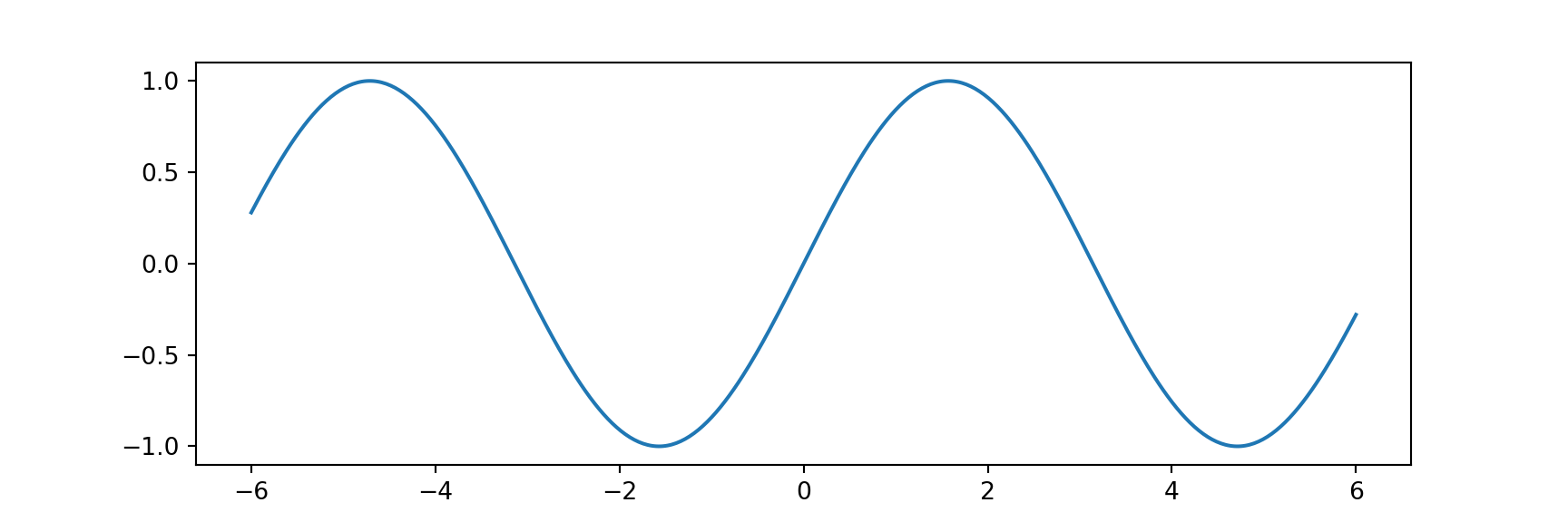
Tricking Out Your Plots

The {matplotlib.pyplot} submodule provides lots of support for customizing your plots.

You can add axes, gridlines, axis labels and titles, plot multiple objects/functions, change colors, fonts, and more!

Example: Below is a code cell that creates a function \(f\left(x\right) = x\cos\left(x\right)\) and plot it with some extras to make the plot more readable.

x_vals = np.linspace(-6, 6, num = 500)
#y_vals = np.sin(x_vals)
def f(x):
  y_vals = x*np.cos(x)
  return y_vals

y_vals = f(x_vals)
plt.figure(figsize = (9, 5))
plt.plot(x_vals, y_vals, color = "purple",
         linewidth = 5)
plt.grid()
plt.axhline(y = 0, color = "black")
plt.axvline(x = 0, color = "black")
plt.title("My function $f(x) = x\cos(x)$",
          fontsize = 36))
plt.xlabel("x", fontsize = 22)
plt.ylabel("y", fontsize = 22)
plt.show()

That’s all for now. Next time, we’ll have a Colab, Python, and \(\LaTeX\) workshop.