MAT 370: Numerical Integration
Newton-Cotes Formulae
March 5, 2026
Reminder: You’ve Seen This Before
Almost surely, integration was introduced to you in a way that was inherently numerical.
Integration was introduced to you as a way to calculate area accumulation.
You broke complex regions into rectangles and noted that the area of the region was approximately the area of the rectangles – more rectangles generally meant better approximation.
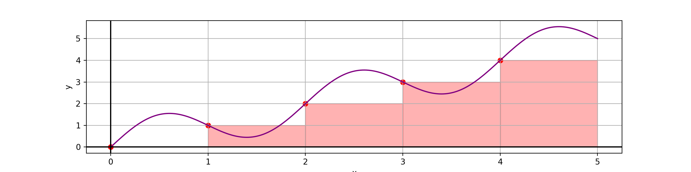
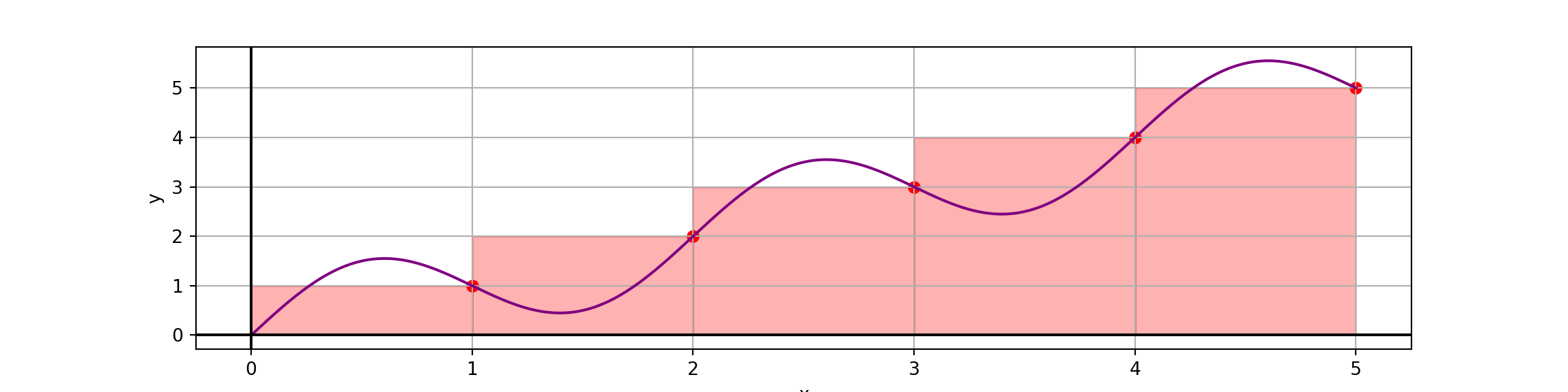
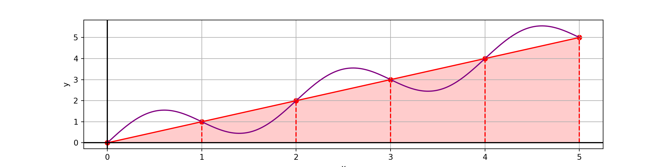
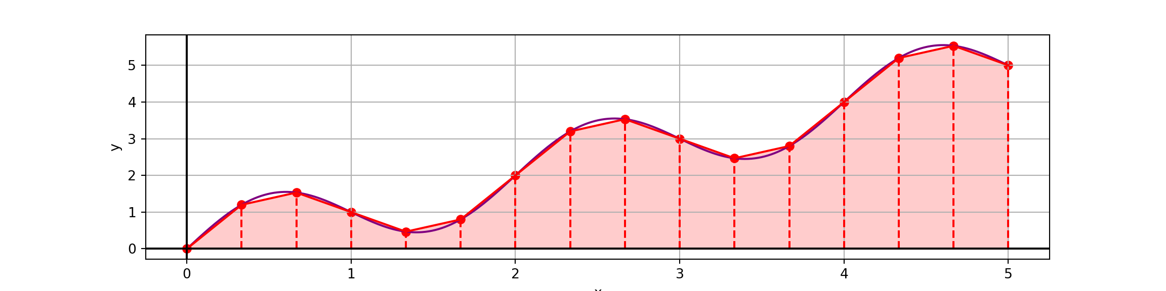
Numerical Integration Strategies
The following table gives several methods which you were probably introduced to in order to approximate \(\displaystyle{\int_{a}^{b}{f\left(x\right)dx}}\), where \(x_0 = a\), \(x_n = b\), and \(x_0 < x_1 < x_2 < \cdots < x_n\).
| Name | Expression for Approximating Integral |
|---|---|
| Left-Endpoint Method | \(\displaystyle{\sum_{i = 0}^{n - 1}{f\left(x_i\right)\Delta x_i}}\) |
| Right-Endpoint Method | \(\displaystyle{\sum_{i = 1}^{n}{f\left(x_i\right)\Delta x_i}}\) |
| Trapezoid Method | \(\displaystyle{\sum_{i = 0}^{n - 1}{\frac{f\left(x_i\right) + f\left(x_{i+1}\right)}{2}\Delta x_i}}\) |
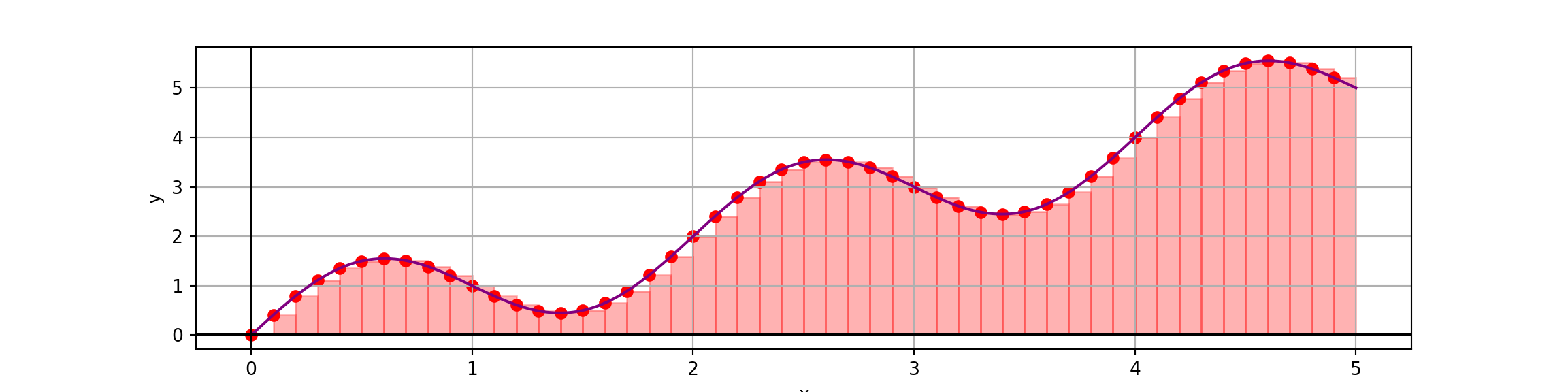
An Example
Example: The picture below shows the trapezoidal rule with \(16\) subintervals being used to approximate \(\displaystyle{\int_{0}^{10}{x + x\sin\left(2x\right)dx}}\). Use the routine defined on the previous slide to compute the estimated area.
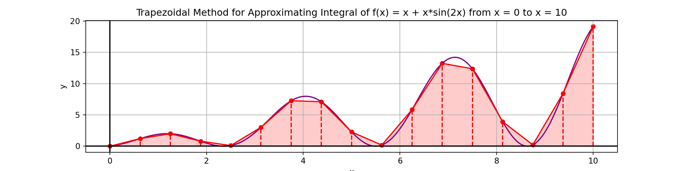
The final estimate for the area was about 48.5 units.
The difference between the previous estimate (8 sub-intervals) and the final one (16 sub-intervals) was still quite large – we haven’t reached convergence yet.
The number of subdivisions I made is  1 , resulting in  2  trapezoids
The difference in approximation between using  1  trapezoids and  2  trapezoids was  -36.42415904042494
The number of subdivisions I made is  2 , resulting in  4  trapezoids
The difference in approximation between using  2  trapezoids and  4  trapezoids was  1.5880685383230997
The number of subdivisions I made is  3 , resulting in  8  trapezoids
The difference in approximation between using  4  trapezoids and  8  trapezoids was  -11.26264765870998
The number of subdivisions I made is  4 , resulting in  16  trapezoids
The difference in approximation between using  8  trapezoids and  16  trapezoids was  -1.0556411183138792
np.float64(48.49288325725569)