MAT 370: Solving Non-Linear Systems

A Multidimensional Newton-Raphson Method

Dr. Gilbert

March 4, 2026

Motivation and Context

You spent an entire semester learning about linear systems and their solutions.

Unfortunately, throw a non-linear system at you, and you’ve got nearly no tools available to your for solving it!

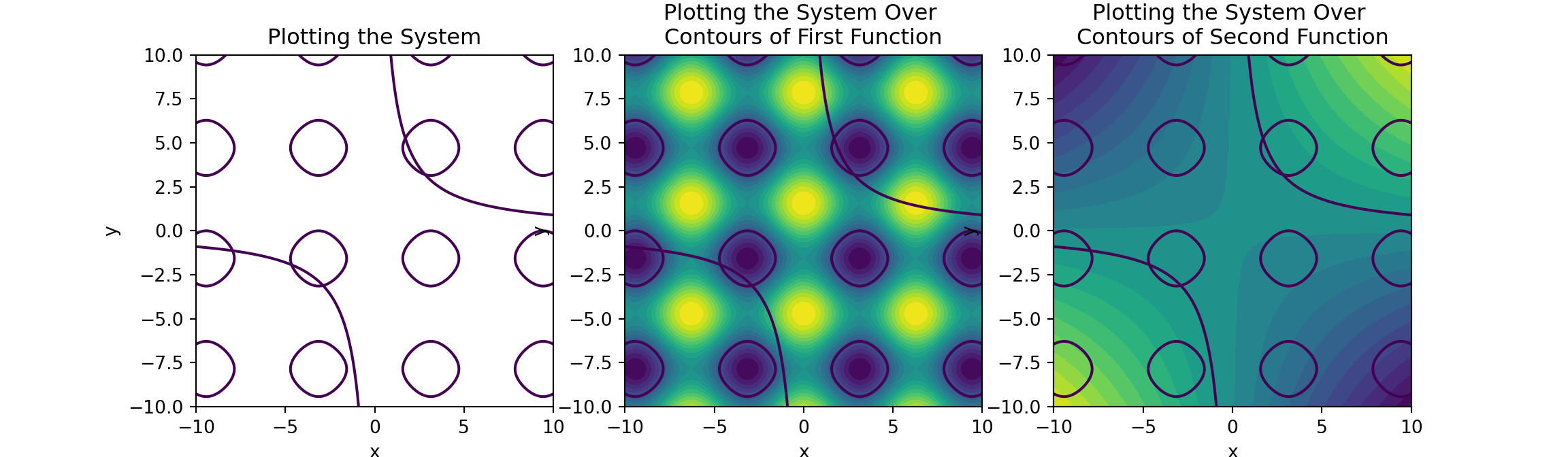
\[\left\{\begin{array}{rcr} \cos\left(x\right) + \sin\left(y\right) + 1 & = & 0\\ xy - 9 & = & 0\end{array}\right.\]

That changes today!

Extending What We’ve Done

In the previous three notebooks we were focused on solving the single equation \(f\left(x\right) = 0\), but there are higher-dimensional versions to consider.

Namely,

\[\vec{f}\left(\vec{x}\right) = \vec{0}\]

which is equivalent to

\[\left\{\begin{array}{lcl} f_1\left(x_1, x_2, \cdots, x_n\right) &= & 0\\ f_2\left(x_1, x_2, \cdots, x_n\right) & = & 0\\ & \vdots &\\ f_n\left(x_1, x_2, \cdots, x_n\right) & = & 0\\ \end{array}\right.\]

• Solving a system like this one is much more difficult than solving a single equation.
• There is no reliable method for bracketing the solution \(\vec{x^*}\).
• This means that we can’t guarantee any algorithm a “good” starting estimate unless there exist some theoretical rationale for the location of the root.

\(\bigstar\) The systems we’re considering now may no longer be linear systems, so we’ll need methods beyond those we encountered earlier in our course.

The Newton-Raphson Method works well with these simultaneous equations, as long as we provide a reasonable starting value.

Deriving a Multidimensional Newton-Raphson Method

Because the math here is in higher dimensions, the details look more complicated.

The foundational idea, though, is the same…

1. Begin from an initial point in space (a reasonable initial guess at the solution).

2. Replace the nonlinear system with its best linear approximation (its Jacobian) at the current point.

   • In the single-variable case, we replaced the curve with its tangent line.
   • Now, we replace the nonlinear map with its local linear approximation.

3. Solve that linear system to determine the update to your previous guess.

4. Using the updated guess, repeat steps 2 and 3 until the estimate for the solution converges within some acceptable tolerance.

Deriving a Multidimensional Newton-Raphson Method

Start with the Taylor Series expansion of \(f_i\left(\vec{x}\right)\) truncated to first degree about the point \(\vec{x^*}\).

\[f_i\left(\vec{x^*} + \Delta\vec{x}\right) \approx f_i\left(\vec{x^*}\right) + \sum_{j = 1}^{n}{\frac{\partial f_i}{\partial x_j}\Delta x_j}\]

Defining the Jacobian Matrix \(J\left(\vec{x^*}\right)\) to be the \(n\times n\) matrix such that \(\displaystyle{J_{ij} = \frac{\partial f_i}{\partial x_j}\left(\vec{x^*}\right)}\) allows us to rewrite the above as the matrix equation:

\[\vec{f}\left(\vec{x^*} + \Delta \vec{x}\right) \approx \vec{f}\left(\vec{x^*}\right) + J\left(\vec{x^*}\right)\Delta\vec{x}\]

With \(\vec{x^*}\) as the previous approximate solution to \(\vec{f}\left(\vec{x}\right) = \vec{0}\), then \(\left(\vec{x^*} + \Delta\vec{x}\right)\) is the improved solution.

To find \(\Delta\vec{x}\), we set \(\vec{f}\left(\vec{x^*} + \Delta\vec{x}\right) = \vec{0}\) and get an approximate solution by solving

\[\begin{align*} \vec{f}\left(\vec{x^*}\right) + J\left(\vec{x^*}\right)\Delta\vec{x} &= 0\\ \implies J\left(\vec{x^*}\right)\Delta\vec{x} &= -\vec{f}\left(\vec{x^*}\right) \end{align*}\]

Implementation Details

So the update requires solving the matrix equation \(\displaystyle{J\left(\vec{x^*}\right)\Delta\vec{x} = -\vec{f}\left(\vec{x^*}\right)}\)

We won’t calculate each \(\displaystyle{\frac{\partial f_i}{\partial x_j}}\) explicitly – instead, we’ll approximate them via the finite difference method (difference quotient).

\[\frac{\partial f_i}{\partial x_j} \approx \frac{f_i\left(\vec{x^*} + \vec{e_j}h\right) - f_i\left(\vec{x^*}\right)}{h}\]

Notice that \(h\) is a “small” step size and \(\vec{e_j}\) is the \(j^{th}\) component identity vector.

Luckily the Newton-Raphson Method is relatively insensitive to small errors in \(J\left(\vec{x}\right)\) – making these approximations is very convenient because we avoid needing to compute and define each partial derivative for the routine.

Writing the Routine

We’re now ready to write the routine.

Just remember, that success of this method depends on having a quality initial estimate for \(\vec{x^*}\) – otherwise, the results are quite unpredictable.

Having some expectation for where the root should occur is necessary because we cannot follow these results blindly.

One more thing – since \(J\left(\vec{x^*}\right) \Delta\vec{x} = - \vec{f}\left(\vec{x^*}\right)\) is system of linear equations, we’ll need access to our gaussPivot() routine from earlier here as well (not shown).

## Jacobian Constructor
def jacobian(f, x, h = 1.0e-4):
  n = len(x)
  jac = np.zeros((n, n))
  f0 = f(x)

  for i in range(n):
    temp = x[i]
    x[i] = temp + h
    f1 = f(x)
    x[i] = temp
    jac[:, i] = (f1 - f0)/h

  return jac, f0

## Newton-Raphson Method for Multiple Dimensions
def newtonRaphsonMultiDim(f, x, tol = 1.0e-9, max_its = 30):
  for i in range(max_its):
    jac, f0 = jacobian(f, x)
    #print("Jacobian \n", jac)
    #print("f0: ", f0)
    if (np.dot(f0, f0)/len(x))**0.5 < tol:
      return x

    dx = gaussPivot(jac, -f0)
    x = x + dx
    if (np.dot(dx, dx))**0.5 < tol*max(max(abs(x)), 1.0):
      return x

  print("Newton-Raphson did not converge.")
  return None

Example Usage

Example 1: Use the Mutli-Dimensional Newton-Raphson routine you just constructed to determine the points of intersection between the circle \(x^2 + y^2 = 3\) and the hyperbola \(xy = 1\).

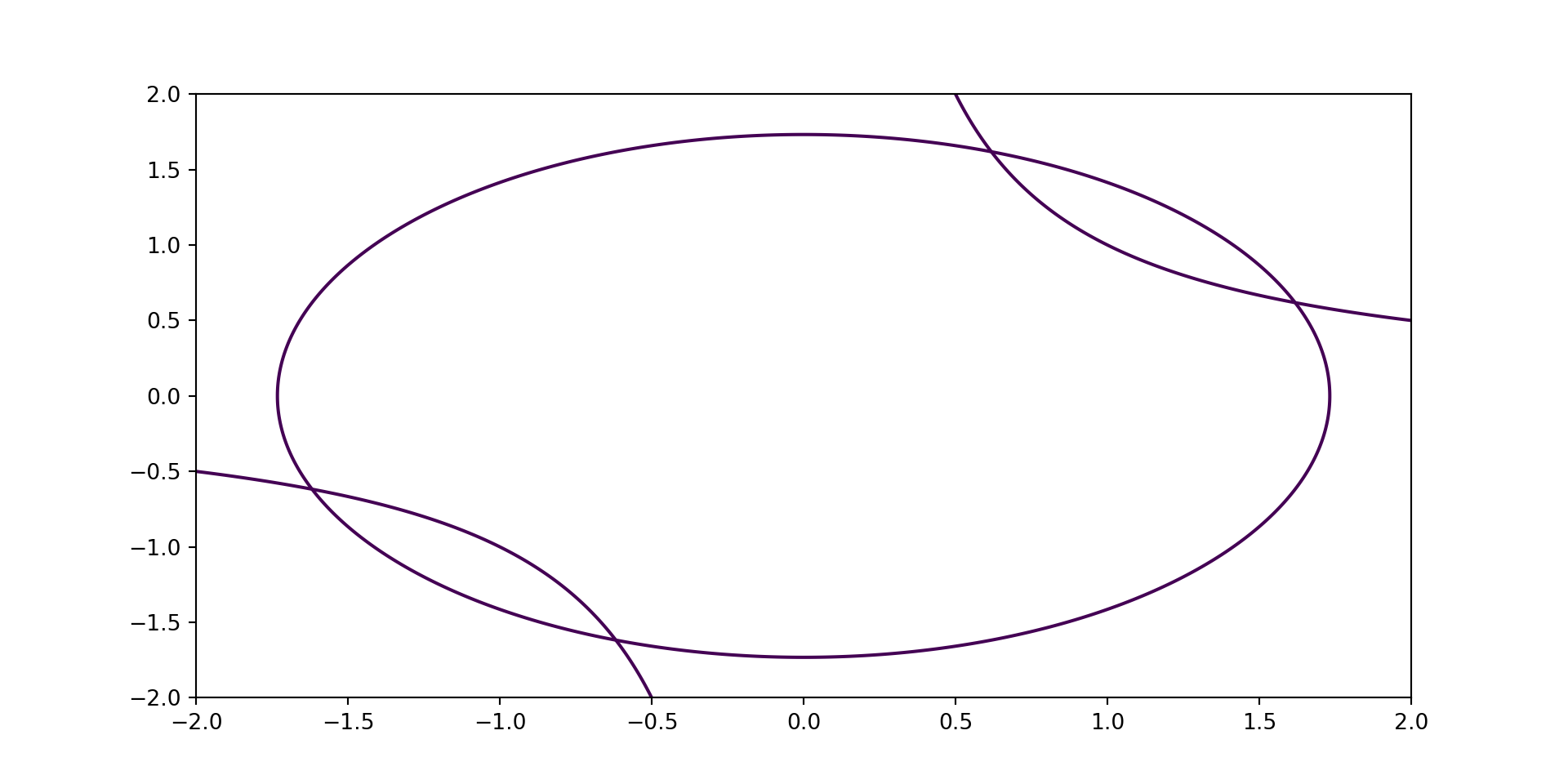
I found the four intersection points to be at:
     [-1.61803399 -0.61803399] (upper left)
     [-0.61803399 -1.61803399] (lower left)
     [0.61803399 1.61803399] (upper right)
     [1.61803399 0.61803399] (lower right)

def f(x):
  F = np.zeros(2)
  F[0] = x[0]**2 + x[1]**2 -3
  F[1] = x[0]*x[1] - 1

  return F

est_upper_left = newtonRaphsonMultiDim(f, [-0.5, 0])
est_lower_left = newtonRaphsonMultiDim(f, [0, -1.5])
est_upper_right = newtonRaphsonMultiDim(f, [0.5, 1.5])
est_lower_right = newtonRaphsonMultiDim(f, [1.5, 0.5])

print("I found the four intersection points to be at:\n", 
      "\t", est_upper_left, "(upper left)\n",
      "\t", est_lower_left, "(lower left)\n",
      "\t", est_upper_right, "(upper right)\n",
      "\t", est_lower_right, "(lower right)")

An Example to Try

Example 2: Find a solution to the system

\[\left\{\begin{array}{rcr} \sin\left(x\right) + y^2 + \ln\left(z\right) - 7 &= 0\\ 3x + 2^y - z^3 + 1 &= 0\\ x + y + z - 5 &= 0\end{array}\right.\]

knowing that a solution exists near \(\left(1, 1, 1\right)\).

Summary and Next Time

• We extended our understanding of the single-variable Newton-Raphson Method to multidimensional, non-linear systems.

  • This is an enormous gain in your ability to solve systems of equations, allowing you to move beyond linear systems only.

• The crux of the idea is to approximate the non-linear system with a local linearization, use that local linearization to identify how to update our current guess, and then to iterate the process until convergence.

• Our implementation is the newtonRaphsonMultiDim() routine, which requires a vector-valued function f that encodes a [perhaps non-linear] system whose constraint vector is \(\vec{0}\), and an initial guess at the solution, x.

  • The trickiest part of using the functionality is creating the vector-valued function.

Next Time: Numerical Differentiation via Finite Difference Approximation