MAT 370: Introduction to Root Finding

Incremental Search and Bisection

Dr. Gilbert

December 30, 2025

Motivation and Context

You’ve spent lots of time over your life solving equations.

At times, it may have felt like you were being asked to memorize “tricks” (though I hope that’s not the case).

You’ve learned how to solve

• Linear equations
• Quadratic equations
• General polynomial equations
• Rational equations
• Exponential equations
• Logarithmic equations
• Trigonometric equations
• And more…

Unfortunately, no matter how good you are with algebraic techniques, they’ll fail you.

Try solving the equation \(\displaystyle{\frac{x^2 - 9}{x + 4}e^x = 10\sin\left(x\right)}\)

No combination of algebraic techniques will permit you to find a solution.

If we reframe the equation as a root-finding problem – that is, find the root of the function \(\displaystyle{f\left(x\right) = \frac{x^2 - 9}{x + 4}e^x - 10\sin\left(x\right)}\), then some additional tools become available to us.

Main Takeaway: Any equation, \(\boxed{~\displaystyle{\text{expression_1} = \text{expression_2}}~}\) can be reframed as a root-finding question for the function \(\boxed{~\displaystyle{f\left(x\right) = \text{expression_1} - \text{expression_2}}~}\)

When Do Functions Have Roots?

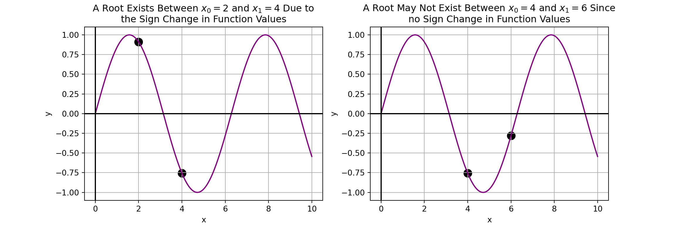
We need a method to determine whether a root exists on an interval. We’ll start with some pictures.

When Do Functions Have Roots?

We need a method to determine whether a root exists on an interval. We’ll start with some pictures.

When Do Functions Have Roots?

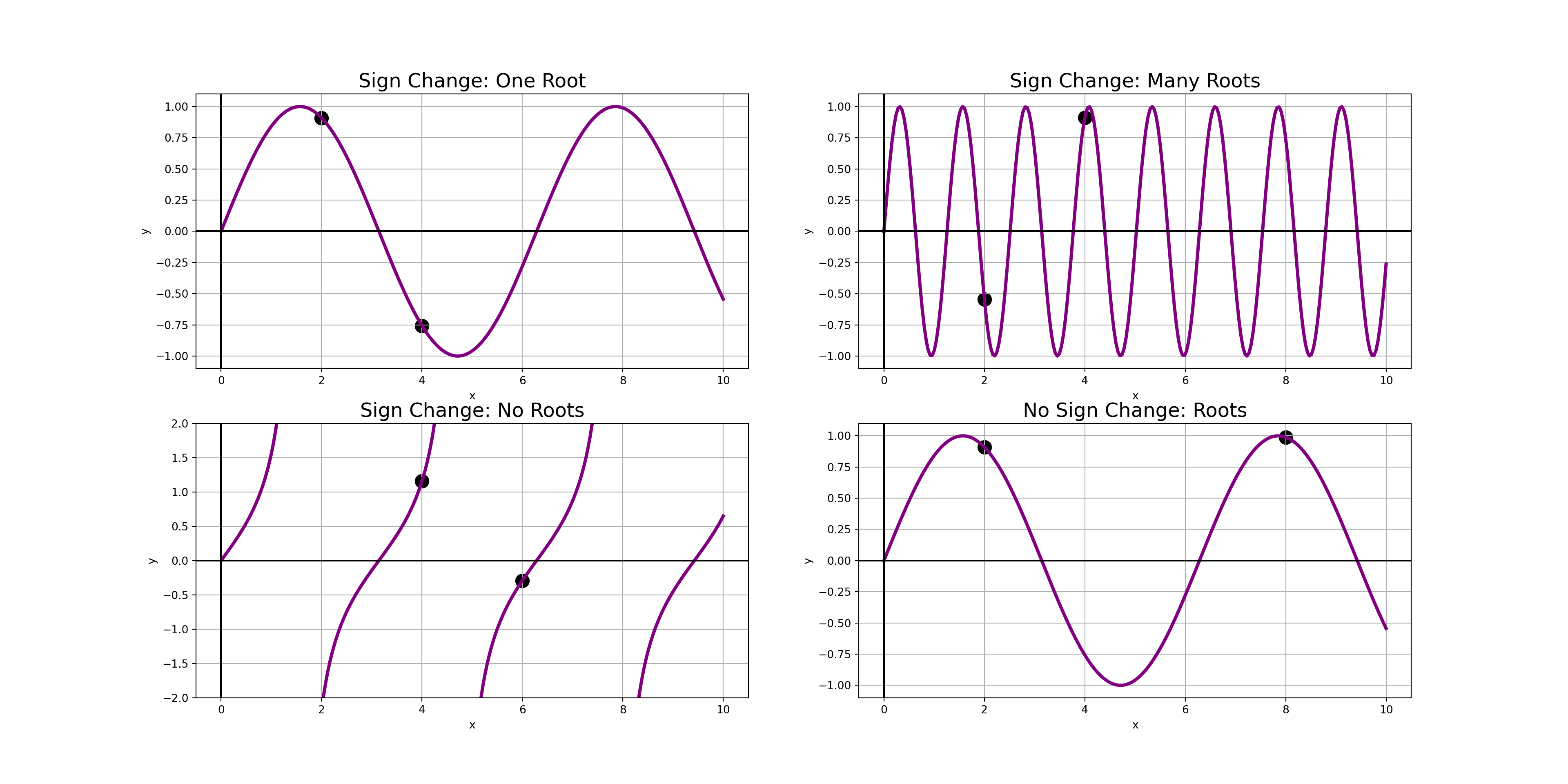
Given the images we’ve seen so far, if we assume that our function is continuous over an interval, then we can find a simple criteria that guarantees the presence of at least one root – a sign change.

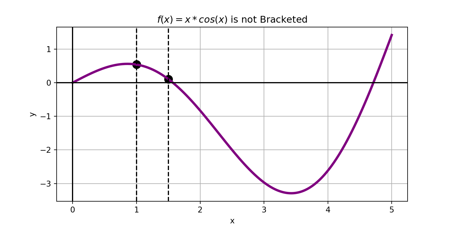
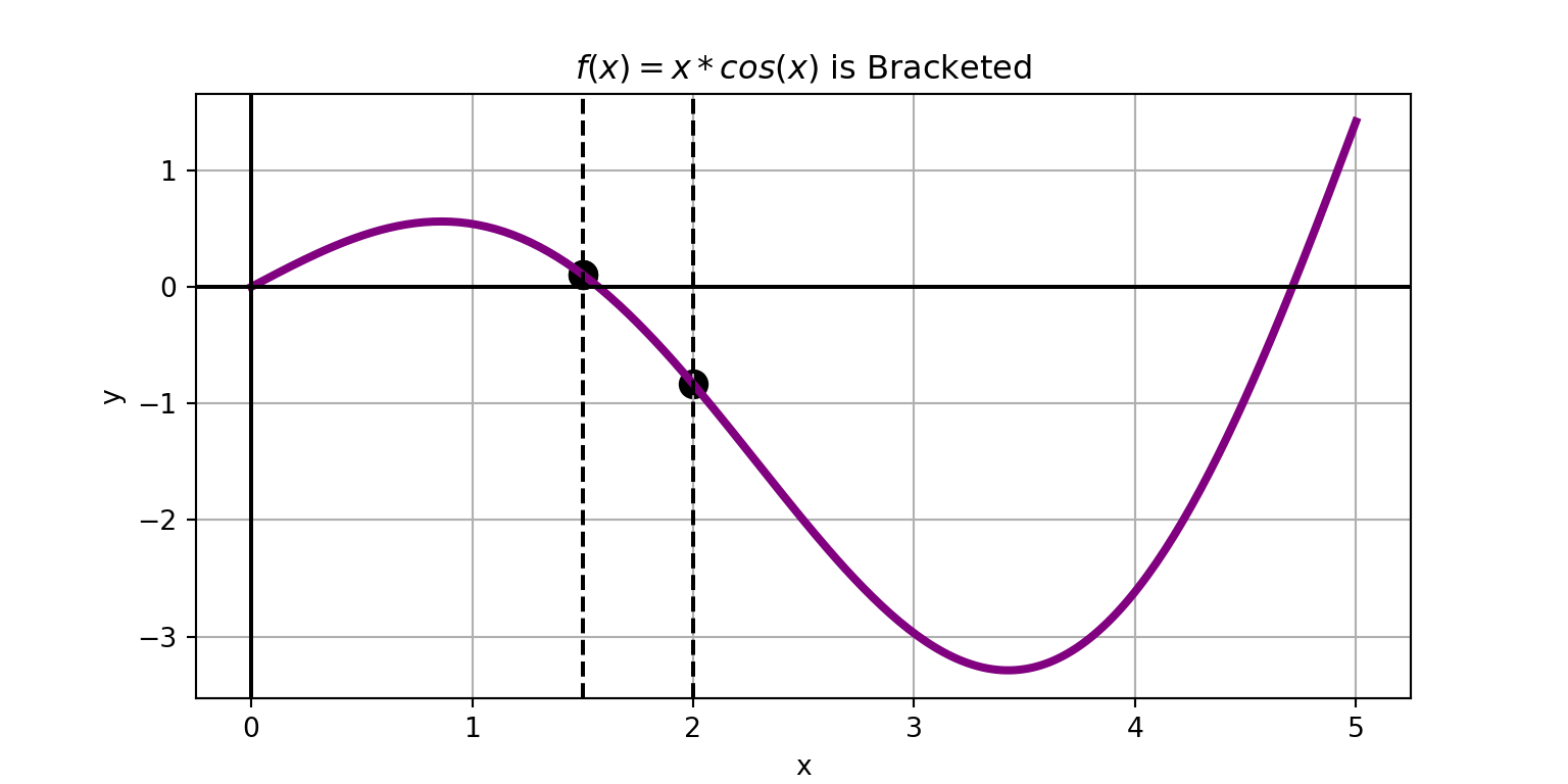
An interval \(\left[a, b\right]\) over which a continuous function \(f\left(x\right)\) experiences a sign change – that is, \(f\left(a\right)\cdot f\left(b\right) < 0\), is called a Bracketed interval.

Continuous functions must have at least one root along and interval over which they are bracketed.

This will be our foundational starting point.

Intuition for Root Finding

If we know that we have a continuous function and an interval that brackets it, then that function has a root on the interval.

Our process will be as follows:

1. Verify that our function is continous (at least along an interval of interest).
2. Discover a bracketing interval for that function.
3. Use a root-finding method to close in on the location of the root.

Finding a Bracketing Interval (Incremental Search)

Since you already know how to identify discontinuities of functions, we’ll start by identifying a strategy for locating a bracketing interval.

The most straight-forward way to discover a bracketing interval is to use a strategy called incremental search.

The idea is simple…

1. Start from the left end of the interval.
2. Take a small step forward.
3. Check for bracketing.
4. Repeat steps 2 and 3 until a bracketed interval is found or you escape the interval of interest.

Finding a Bracketing Interval (Incremental Search)

Since you already know how to identify discontinuities of functions, we’ll start by identifying a strategy for locating a bracketing interval.

The most straight-forward way to discover a bracketing interval is to use a strategy called incremental search.

The idea is simple…

1. Start from the left end of the interval.
2. Take a small step forward.
3. Check for bracketing.
4. Repeat steps 2 and 3 until a bracketed interval is found or you escape the interval of interest.

Finding a Bracketing Interval (Incremental Search)

Since you already know how to identify discontinuities of functions, we’ll start by identifying a strategy for locating a bracketing interval.

The most straight-forward way to discover a bracketing interval is to use a strategy called incremental search.

The idea is simple…

1. Start from the left end of the interval.
2. Take a small step forward.
3. Check for bracketing.
4. Repeat steps 2 and 3 until a bracketed interval is found or you escape the interval of interest.

Finding a Bracketing Interval (Incremental Search)

Since you already know how to identify discontinuities of functions, we’ll start by identifying a strategy for locating a bracketing interval.

The most straight-forward way to discover a bracketing interval is to use a strategy called incremental search.

The idea is simple…

1. Start from the left end of the interval.
2. Take a small step forward.
3. Check for bracketing.
4. Repeat steps 2 and 3 until a bracketed interval is found or you escape the interval of interest.

Finding a Bracketing Interval (Incremental Search)

Since you already know how to identify discontinuities of functions, we’ll start by identifying a strategy for locating a bracketing interval.

The most straight-forward way to discover a bracketing interval is to use a strategy called incremental search.

The idea is simple…

1. Start from the left end of the interval.
2. Take a small step forward.
3. Check for bracketing.
4. Repeat steps 2 and 3 until a bracketed interval is found or you escape the interval of interest.

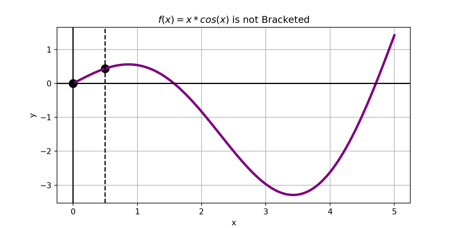
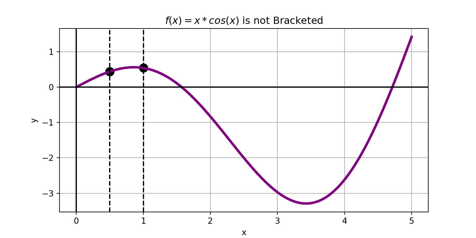
The function \(f\left(x\right) = x\cos\left(x\right)\) is bracketed on the interval \(\left[1.5, 2\right]\).

An Example (By Hand)

Example: Given the function \(f\left(x\right) = x^2 - 3x + 1\), use incremental search over the interval \(\left[0, 1\right]\) with \(dx = 0.2\) to determine whether a root may exist on the interval.

Comments on Incremental Search

• The result of incremental search is a bracketed interval of the form \(\left[x_1, x_2\right]\) within which a root of the function exists.

• The step size used determines the width of the bracketed interval returned.

  • Using a very small step size returns a very narrow interval.
  • Using a very large step size returns a very wide interval, or may even skip over the root altogether!

• Using extremely small step sizes is not efficient and may cause incremental search to run for a very large number of iterations before finding the bracketed interval.

  • This may be unacceptable.
  • There are much faster methods for converging on the root once we know we have a bracketed interval anyway.

• Your goal with incremental search should simply be to find a bracketed interval and then move on to a more efficient root-finding method to close in.

Implementing Incremental Search

def incrementalSearch(f, a, b, dx):
  #Write the Incremental Search function here.
  x1 = a
  x2 = x1 + dx

  while (np.sign(f(x1)) == np.sign(f(x2))) and (x2 <= b):
    x1 = x2
    x2 = x1 + dx

  if np.sign(f(x1)) != np.sign(f(x2)):
    return [x1, x2]

  print("I didn't find a bracketed interval.")
  return None

Example 1: Use the incrementalSearch() routine on the interval \(\left[0, 2\right]\) with \(f\left(x\right) = x\cdot\cos\left(x\right)\) and \(dx = 0.1\).

Example 2: Use incrementalSearch() to find the root of the function \(\displaystyle{f\left(x\right) = \frac{x^2 - 9}{x + 4}e^x - 10\sin\left(x\right)}\) which lies on the interval \(\left[0, 5\right]\).

Increasing Accuracy

We’ll find better methods for closing in on the location of a root. However, it is possible to close in using incrementalSearch() by using progressively smaller step sizes on the bracketed intervals being found.

def f(x):
  return x*np.cos(x)

x1 = 0.1
x2 = 2

tic = time.time()

for i in range(6):
  dx = 0.1**(i+1)
  x1, x2 = incrementalSearch(f, x1, x2, dx)

toc = time.time()

print(x1, x2)

1.5707960000000003 1.5707970000000002

print("That took ", toc - tic, " seconds")

That took  0.0017800331115722656  seconds

def f(x):
  return x*np.cos(x)

x1 = 0.1
x2 = 2
dx = 0.000001

tic = time.time()

x1, x2 = incrementalSearch(f, x1, x2, dx)

toc = time.time()

print(x1, x2)

1.5707959999608814 1.5707969999608813

print("That took ", toc - tic, " seconds")

That took  2.608621835708618  seconds

Closing in on a Root: Bisection

We’ll find multiple methods for closing in on the root of a function once we have a bracketed interval for it.

Our first method is the simplest and is reasonably effective.

Using the method of Bisection, we find the midpoint of our bracketed interval, evaluate the function at both endpoints and the midpoint, identify which subinterval remains bracketed, and then shrink down to that subinterval.

We continue doing this until (i) we obtain a function value of exactly \(0\), or (ii) the resulting subinterval is smaller than some pre-set tolerance for error.

If we reach this second condition, then we compute the midpoint once more and report that value as the numerical approximation of the root.

Example: The function \(\displaystyle{f\left(x\right) = x^2 - 5x + 3}\) has a root on the interval \(\left[0, 2\right]\). Verify that this interval is bracketed, and then carry out four iterations of the bisection method to approximate the value of the root. Determine the level of accuracy that you’ve obtained through this procedure.

Implementing Bisection

def bisection(f, x1, x2, tol = 1.0e-9):
  dx = x2 - x1
  y1 = f(x1)
  y2 = f(x2)

  if np.sign(y1) == np.sign(y2):
    print("The interval [x1, x2] is not bracketed. \nPlease provide a bracketed interval to start.")
    return None

  while dx > tol:
    x3 = (x1 + x2)/2
    y3 = f(x3)

    if np.sign(y1) == np.sign(y3):
      x1 = x3
    else:
      x2 = x3

    y1 = f(x1)
    y2 = f(x2)
    dx = dx/2

  x = (x1 + x2)/2
  return x

Example: Use our Bisection function to approximate the root of the function \(f\left(x\right) = x\cdot \cos\left(x\right)\) in the bracketed interval \(\left[1, 2\right]\).

Example: Use bisection to find the root of the function \(f\left(x\right) = \frac{x^2 - 9}{x + 4}e^x - 10\sin\left(x\right)\) which lies on the interval \(\left[2, 4\right]\).

Example: The natural frequencies of a uniform cantilever beam are related to the roots \(\beta_i\) of the frequency equation \(f\left(\beta\right) = \cosh\left(\beta\right)\cos\left(\beta\right) + 1\), where

\[\begin{align*} \beta_i^4 &= \left(2\pi f_i\right)^2\frac{\tt{m}\tt{L}^3}{\tt{E}\tt{I}}\\ f_i &= i^{th}~\text{natural frequency ($\tt{cps}$)}\\ m &= ~\text{mass of the beam}\\ L &= ~\text{Length of the beam}\\ E &= ~\text{modulus of elasticity}\\ I &= ~\text{moment of inertia of the cross section} = \displaystyle{\frac{1}{12}\left(\text{width}\right)\left(\text{height}^3\right)} \end{align*}\]

Determine the lowest two frequencies of a steel beam \(0.9~\tt{m}\) long, with rectangular cross-sections \(25~\tt{mm}\) wide and \(2.5~\tt{mm}\) high. The mass-density of steel is \(7580~\tt{kg/m}^3\) and \(E = 200~\text{GPa}\).

Summary

• In this notebook, we introduced and implemented the method of incremental search for locating bracketed intervals, and also the bisection method for quickly closing in on the location of a root on the interior of a bracketed interval.
• These techniques can be utilized to solve equations of the form \(f\left(x\right) = 0\) for any function given some initial search interval.

Next Time: In the next notebook we’ll look at series of techniques called linear interpolation which complement the bisection method we encountered here.