MAT 370: Cubic Spline Interpolants
February 17, 2026
Motivation and Context
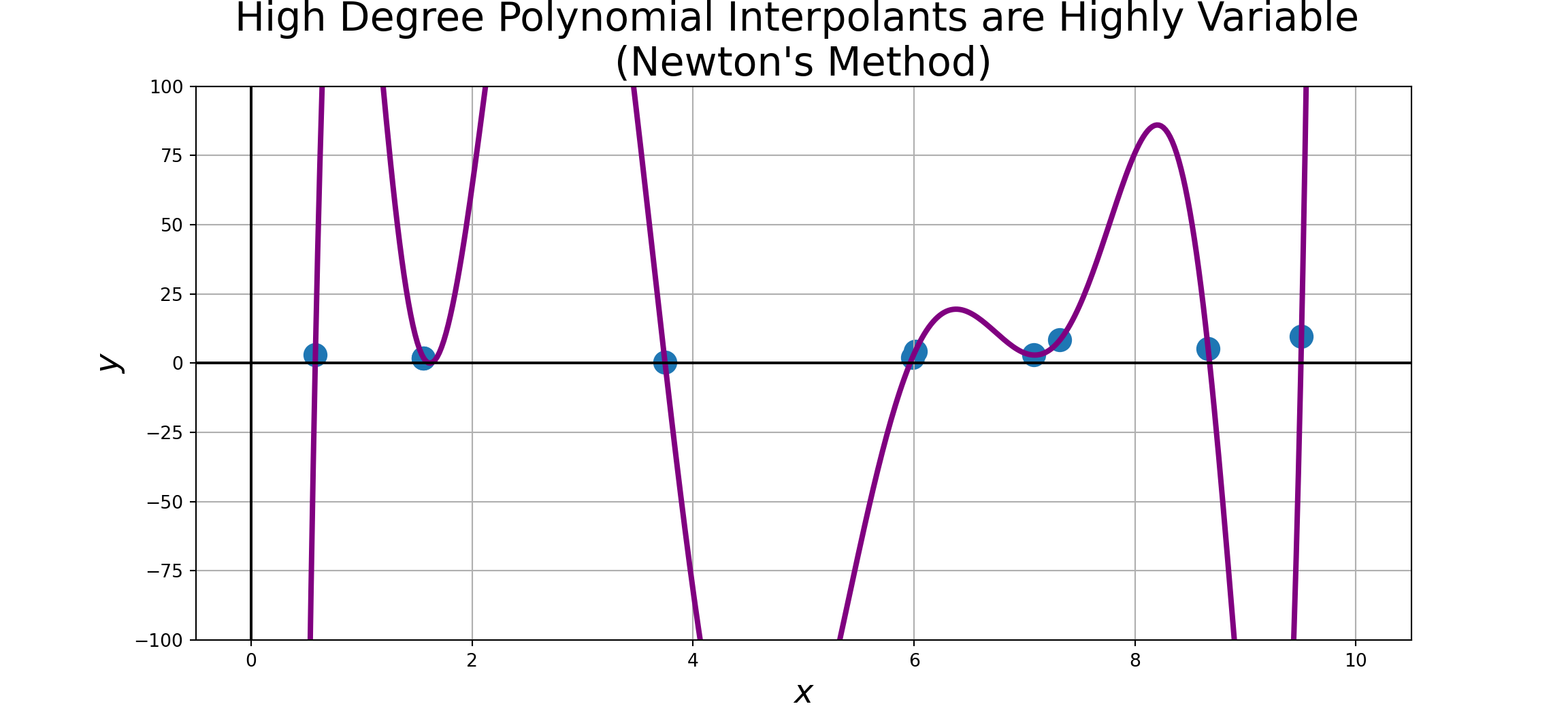
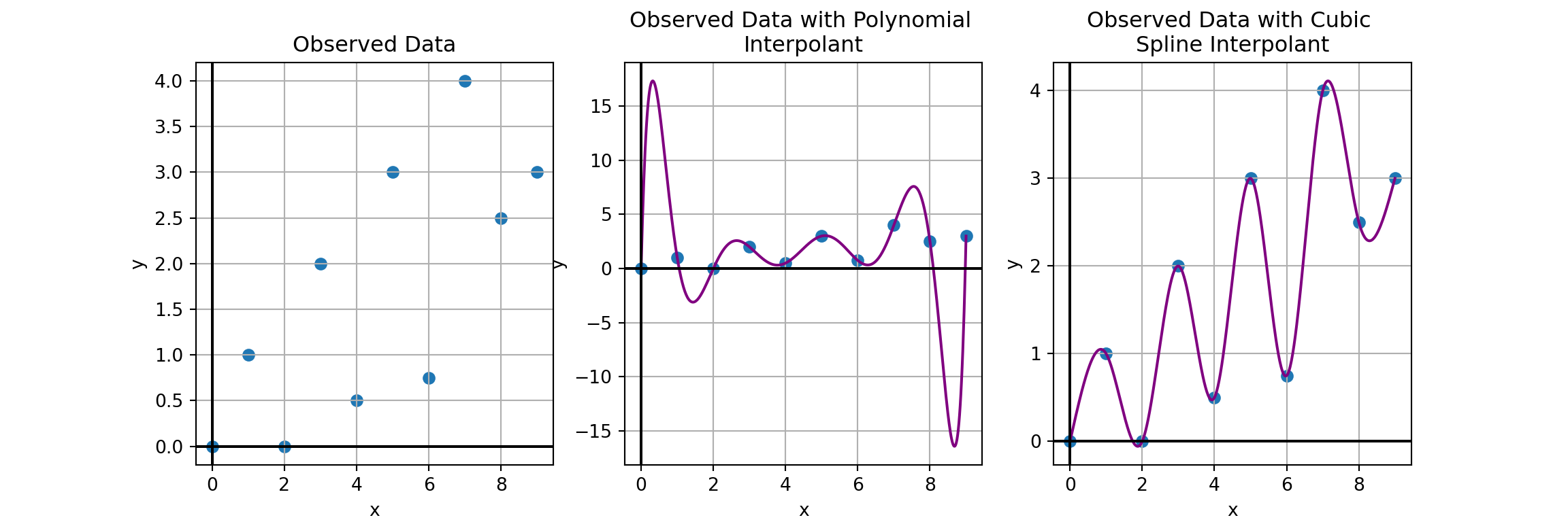
At the end of our last discussion, we saw that increasing the number of observed data points also increases the degree of the polynomial.
High degree polynomials invite greater levels of variability between control points, especially near the boundaries of the observed region.
Constraints: Natural Cubic Splines
Since our elastic strips satisfy \(\frac{d^4\omega}{dx^4} = 0\), we know that the strips are cubic polynomials.
We impose a few additional constraints on our cubic splines as well.
- The slope (first derivative) is continuous through each pin.
- The curvature (second derivative) is continuous through each pin.
- The curvature at the left-most and right-most pins is \(0\).
Because of these constraints, our cubic splines will have much more controlled behavior.
Using the Interpolant
Example: Use the cubic spline interpolator we just constructed to build a cubic spline interpolant for the observed data to the right.
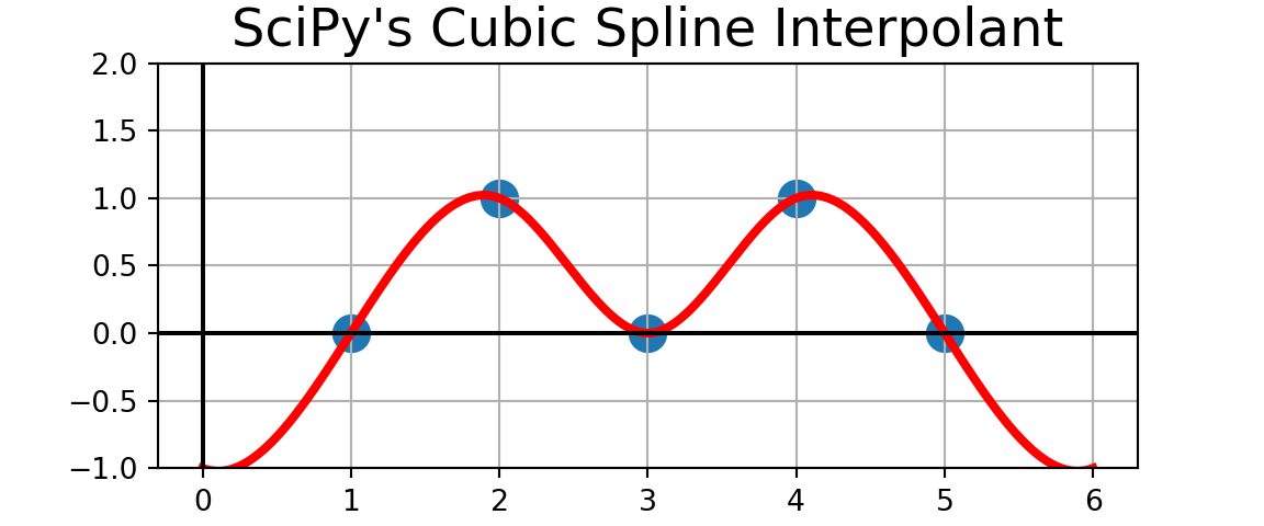
If you like, compare your cubic spline interpolant to the one produced by CubicSpline() from scipy.interpolate. Before executing the code to compare, what do you expect to see?
| x | y |
|---|---|
| 1 | 0 |
| 2 | 1 |
| 3 | 0 |
| 4 | 1 |
| 5 | 0 |
x = np.array([1.0, 2, 3, 4, 5])
y = np.array([0.0, 1, 0, 1, 0])

x_new = np.linspace(0, 6, 10000)

k = curvatures(x, y)

y_new = x_new.copy()
for j in range(len(x_new)):
  y_new[j] = evalSpline(x, y, k, x_new[j])

plt.figure(figsize = (6,2))
plt.scatter(x, y, s = 150)
plt.plot(x_new, y_new, color = "purple", linewidth = 3)
plt.grid()
plt.axvline(color = "black")
plt.axhline(color = "black")
plt.title("Our Cubic Spline Interpolant", fontsize = 18)
plt.ylim((-1, 2));
plt.show()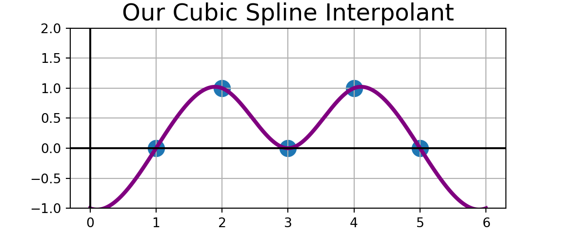

Using the Interpolant
Example: Use the cubic spline interpolator we just constructed to build a cubic spline interpolant for the observed data to the right.
If you like, compare your cubic spline interpolant to the one produced by CubicSpline() from scipy.interpolate. Before executing the code to compare, what do you expect to see? They’re the same!
| x | y |
|---|---|
| 1 | 0 |
| 2 | 1 |
| 3 | 0 |
| 4 | 1 |
| 5 | 0 |
x = np.array([1.0, 2, 3, 4, 5])
y = np.array([0.0, 1, 0, 1, 0])

x_new = np.linspace(0, 6, 10000)

k = curvatures(x, y)

y_new = x_new.copy()
for j in range(len(x_new)):
  y_new[j] = evalSpline(x, y, k, x_new[j])

plt.figure(figsize = (6,2))
plt.scatter(x, y, s = 150)
plt.plot(x_new, y_new, color = "purple", linewidth = 3)
plt.grid()
plt.axvline(color = "black")
plt.axhline(color = "black")
plt.title("Our Cubic Spline Interpolant", fontsize = 18)
plt.ylim((-1, 2));
plt.show()
Comments on the Interpolant
This is the first time we have a routine which is split across multiple functions without a complete wrapper for the entire process (though you could build one).
The
curvatures()function solves the tridiagonal system which we discovered through the math on the previous slides.The
findSegment()function is a helper function for evaluating the cubic spline interpolant.The
evalSpline()function is the one you’ll use to take new input values and to evaluate the cubic spline interpolants and obtain outputs.