MAT 350: Pivots and their Impact on Solutions
September 22, 2025
Warm-Up Problems
Examples: Reduce the following matrices to their equivalent reduced row echelon forms (RREF).
\[i)~~~~\begin{bmatrix} 1 & -1 & -1\\ 3 & -3 & -2\end{bmatrix}~~~~~~~~~~~~ii)~~~~\begin{bmatrix} 19 & -6 & -24 & 0\\ 6 & -2 & -8 & 0\\ -18 & 6 & 24 & 1\end{bmatrix}\]
Reminders and Today’s Goal
- Over the previous meetings, we’ve discussed augmented coefficient matrices and their connection to linear systems.
- We’ve seen that we can use our three permissible row-reduction operations to obtain solutions to our linear systems.
- An augmented matrix in row echelon form \[\small{\left[\begin{array}{cccc|c} \blacksquare & * & \cdots & * & b_1\\ 0 & \blacksquare & \cdots & * & b_2\\ \vdots & \vdots & \ddots & \vdots & \vdots\\ 0 & 0 & \cdots & \blacksquare & b_n\end{array}\right]}\]
- An augmented matrix in reduced row echelon form \[\left[\begin{array}{cccc|c} \boxed{~1~} & 0 & \cdots & 0 & b_1\\ 0 & \boxed{~1~} & \cdots & 0 & b_2\\ \vdots & \vdots & \ddots & \vdots & \vdots\\ 0 & 0 & \cdots & \boxed{~1~} & b_n\end{array}\right]\]
Reminders and Today’s Goal
- An augmented matrix in row echelon form \[\small{\left[\begin{array}{cccc|c} \blacksquare & * & \cdots & * & b_1\\ 0 & \blacksquare & \cdots & * & b_2\\ \vdots & \vdots & \ddots & \vdots & \vdots\\ 0 & 0 & \cdots & \blacksquare & b_n\end{array}\right]}\]
- An augmented matrix in reduced row echelon form \[\left[\begin{array}{cccc|c} \boxed{~1~} & 0 & \cdots & 0 & b_1\\ 0 & \boxed{~1~} & \cdots & 0 & b_2\\ \vdots & \vdots & \ddots & \vdots & \vdots\\ 0 & 0 & \cdots & \boxed{~1~} & b_n\end{array}\right]\]
The black boxes and boxed elements are called pivots and their location tells us about the solution spaces of the corresponding systems.
Reminder: Pivots do not necessarily occur on the diagonal, and it is not the case that every row or every column of the matrix must have a pivot.
Goal: Determine what and how the number and location of pivots in a matrix in row echelon form tell us about the solution space.
Pivots and Solution Spaces
We first saw pivots in our Day 4 notebook.
pivots are the leading non-zero entries in each row of a matrix in row echelon form.
- A row in a matrix containing a pivot is called a pivot row.
- A column containing a pivot is called a pivot column.
We identified that the positions of our pivots determine the size of our solution space corresponding to a linear system.
- If the rightmost column of the augmented coefficient matrix is a pivot column, then the system is inconsistent (it has no solutions).
- If all columns other than the rightmost column of the augmented matrix are pivot columns, then the system is consistent and has a unique solution.
- If at least one column other than the rightmost column of the augmented coefficient matrix is not a pivot column, then the system has infinitely many solutions.
Pivots and Solution Spaces
- If the rightmost column of the augmented coefficient matrix is a pivot column, then the system is inconsistent (it has no solutions).
- If all columns other than the rightmost column of the augmented matrix are pivot columns, then the system is consistent and has a unique solution.
- If at least one column other than the rightmost column of the augmented coefficient matrix is not a pivot column, then the system has infinitely many solutions.
Example: The locations of the pivots in the augmented coefficient matrices below tell us about the size of the corresponding solution spaces.
\[\overset{\text{Unique Solution}}{\left[\begin{array}{cc|c}\boxed{~1~} & 0 & -3\\ 0 & \boxed{~1~} & 2\end{array}\right]}~~~~\overset{\text{No Solutions}}{\left[\begin{array}{cc|c}\boxed{~1~} & 0 & -3\\ 0 & 0 & \boxed{~1~}\end{array}\right]}~~~~\overset{\text{Infinitely Many Solutions}}{\left[\begin{array}{cc|c}\boxed{~1~} & 0 & -3\\ 0 & 0 & 0\end{array}\right]}\]
Fundamental Observations About Pivots
Limitations on Number of Pivots: Recognizing come obvious limitations can reduce the amount of work we need to do if we are only interested in existence or particularly uniqueness of solutions to systems.
In any \(m\times n\) matrix, there can be at most one pivot per row.
- That is, the number of pivots is at most \(m\).
Similarly, in any \(m\times n\) matrix, there can be at most one pivot per column.
- That is, the number of pivots is at most \(n\).
Example: If an augmented coefficient matrix is \(4\times 7\) (so the coefficient matrix is \(4\times 6\)), then the maximum number of pivots in the augmented coefficient matrix is \(4\).
Fundamental Observations About Pivots
Limitations on Number of Pivots: Recognizing come obvious limitations can reduce the amount of work we need to do if we are only interested in existence or particularly uniqueness of solutions to systems.
In any \(m\times n\) matrix, there can be at most one pivot per row.
- That is, the number of pivots is at most \(m\).
Similarly, in any \(m\times n\) matrix, there can be at most one pivot per column.
- That is, the number of pivots is at most \(n\).
Example: If an augmented coefficient matrix is \(4\times 7\) (so the coefficient matrix is \(4\times 6\)), then the maximum number of pivots in the augmented coefficient matrix is \(4\). This means that not every column in the coefficient matrix can be a pivot column. For this reason, the corresponding system cannot have a unique solution – it is either an inconsistent system or it has infinitely many solutions.
Pivots, Basic Variables, and Free Variables
- The locations of pivots in a row echelon form matrix tell us about the number of solutions to the corresponding linear system.
- The pivots tell us about the roles of the variables in the corresponding solution set.
In an augmented coefficient matrix, each column to the left of the augmentation line corresponds to a variable in the system.
\[\left[\begin{array}{cccc|c} \overset{\mathbf{x_1}}{a_{11}} & \overset{\mathbf{x_2}}{a_{12}} & \cdots & \overset{\mathbf{x_n}}{a_{1n}} & b_1\\ a_{21} & a_{22} & \cdots & a_{2n} & b_2\\ \vdots & \vdots & \ddots & a_{1n} & \vdots\\ a_{m1} & a_{m2} & \cdots & a_{mn} & b_m\end{array}\right]\]
Pivots, Basic Variables, and Free Variables
In an augmented coefficient matrix, each column to the left of the augmentation line corresponds to a variable in the system.
\[\left[\begin{array}{cccc|c} \overset{\mathbf{x_1}}{a_{11}} & \overset{\mathbf{x_2}}{a_{12}} & \cdots & \overset{\mathbf{x_n}}{a_{1n}} & b_1\\ a_{21} & a_{22} & \cdots & a_{2n} & b_2\\ \vdots & \vdots & \ddots & a_{1n} & \vdots\\ a_{m1} & a_{m2} & \cdots & a_{mn} & b_m\end{array}\right]\]
If a variable corresponds to a pivot column, then that variable is a basic variable.
- The values of basic variables are determined.
If a variable does not correspond to a pivot column, then that variable is a free variable.
- Free variables can take on any value.
Remark: Once the values for all free variables have been chosen, then the values of the basic variables are determined.
Recap: Pivots, Basic Variables, Free Variables, and Solutions Sets
- Columns to the left of the augmenting line in an augmented coefficient matrix correspond to variables in the system.
- Pivots are the leftmost non-zero entries in each row.
- Rows and columns containing pivots are called pivot rows and pivot columns respectively.
- If the rightmost column of an augmented coefficient matrix is a pivot column, then the corresponding linear system is inconsistent – it has no solutions. Otherwise, the system is consistent and either has a unique solution, or infinitely many solutions.
- Any variable in a system corresponding to a column which is not a pivot column in the augmented coefficient matrix is a free variable – it can take on any value and the system will remain consistent.
Recap: Pivots, Basic Variables, Free Variables, and Solution Sets
- Any variable in a system corresponding to a pivot column in the augmented coefficient matrix is a basic variable – its value will be completely determined once values for any free variables have been chosen.
- If a consistent system has at least one free variable, then it has infinitely many solutions.
- If a consistent system has no free variables, then it has a unique (exactly one) solution.
Examples to Try
Example: For each of the augmented coefficient matrices below, determine the following:
- Is the matrix in reduced row echelon form, row echelon form, or neither?
- Identify the locations of the pivots.
- Decide whether the corresponding linear system is consistent or inconsistent.
- For any consistent linear systems, identify whether the system has any free variables, and identify them if so.
- Identify the size of the solution space for any consistent linear systems you’ve found.
\[\small{(A)~~\left[\begin{array}{ccc|c} 1 & 0 & 0 & 2\\ 0 & 1 & 0 & -1\\ 0 & 0 & 1 & 3\end{array}\right]}\] \[\small{(B)~~\left[\begin{array}{ccc|c} 1 & 2 & -1 & 3\\ 0 & 1 & 4 & -2\\ 0 & 0 & 0 & 0\end{array}\right]}~~~\small{(C)~~\left[\begin{array}{cc|c} 0 & 1 & 2\\ 1 & 0 & 3\end{array}\right]}\]
\[\small{(D)~~\left[\begin{array}{ccc|c} 1 & 2 & -1 & 0\\ 0 & 1 & 3 & 2\\ 1 & 3 & 2 & 7\end{array}\right]}\] \[\small{(E)~~\left[\begin{array}{cccc|c} 1 & 0 & -2 & 4 & 1\\ 0 & 1 & 3 & -1 & 0\end{array}\right]}\]
Parametric Vector Form and Geometry
Linear Systems and Matrix Equations: Converting a linear system into an augmented coefficient matrix really converts the system to an equivalent matrix equation \(A\vec{x} = \vec{b}\) which we solve instead.
The solution to such a matrix equation is a vector. Because of this, it is often convenient to write solutions to systems of linear equations as vectors.
Example: The linear system \(\left\{\begin{array}{rcr} x_1 - 2x_2 + x_3 & = & -5\\ 2x_2 + 3x_3 & = & 9\end{array}\right.\) corresponds to the matrix equation \(\begin{bmatrix} 1 & -2 & 1\\ 0 & 2 & 3\end{bmatrix}\begin{bmatrix} x_1\\ x_2\\ x_3\end{bmatrix} = \begin{bmatrix} -5\\ 9\end{bmatrix}\)
Parametric Vector Form and Geometry
\[\overset{\text{Linear System}}{\left\{\begin{array}{lcl} a_{11}x_1 + a_{12}x_2 + \cdots a_{1n}x_n & = & b_1\\ a_{21}x_1 + a_{22}x_2 + \cdots a_{2n}x_n & = & b_1\\ & \vdots & \\ a_{m1}x_1 + a_{m2}x_2 + \cdots a_{mn}x_n & = & b_m \end{array}\right.}~~~~~~~~\overset{\text{Matrix Equation}}{\begin{bmatrix} a_{11} & a_{12} & \cdots & a_{1n}\\ a_{21} & a_{22} & \cdots & a_{2n}\\ \vdots & \cdots & \ddots & \vdots\\ a_{m1} & a_{m2} & \cdots & a_{mn}\end{bmatrix}\vec{x} = \begin{bmatrix} b_1\\ b_2\\ \vdots\\ b_m\end{bmatrix}}\]
When a linear system has a solution with free variables, the solution vector to the corresponding matrix equation \(A\vec{x} = \vec{b}\) will not be completely determined
- Free variables show up as parameters within the solution vector.
- We can express the solution vector as a sum of a constant vector and one or more directional vectors scaled by parameters (the free variables).
- This process is called writing the solution in parametric vector form.
Parametric Vector Form and Geometry: Example
Example: Consider the augmented coefficient matrix \(\left[\begin{array}{ccc|c} 1 & -2 & 1 & -5\\ 0 & 2 & 3 & 9\end{array}\right]\), which has reduced row echelon form \(\left[\begin{array}{ccc|c} 1 & 0 & 4 & 4\\ 0 & 1 & 3/2 & 9/2\end{array}\right]\).
- \(x_1\) and \(x_2\) are basic variables, but \(x_3\) is a free variable because the third column of the augmented coefficient matrix is not a pivot column.
- Both \(x_1\) and \(x_2\) depend on the free variable \(x_3\).
Parametric Vector Form and Geometry: Example
Example: Consider the augmented coefficient matrix \(\left[\begin{array}{ccc|c} 1 & -2 & 1 & -5\\ 0 & 2 & 3 & 9\end{array}\right]\), which has reduced row echelon form \(\left[\begin{array}{ccc|c} 1 & 0 & 4 & 4\\ 0 & 1 & 3/2 & 9/2\end{array}\right]\).
- We can write the solution vector as \(\vec{x} = \begin{bmatrix} 4 - 4x_3\\ \frac{9}{2} - \frac{3}{2}x_3\\ x_3\end{bmatrix}\)
- However, this masks the structure of the solution space.
- Decomposing the solution vector into a constant vector plus a directional vector with respect to the parameter (free variable) \(x_3\) provides additional insight.
Parametric Vector Form and Geometry: Example
Example: Consider the augmented coefficient matrix \(\left[\begin{array}{ccc|c} 1 & -2 & 1 & -5\\ 0 & 2 & 3 & 9\end{array}\right]\), which has reduced row echelon form \(\left[\begin{array}{ccc|c} 1 & 0 & 4 & 4\\ 0 & 1 & 3/2 & 9/2\end{array}\right]\).
- Decomposing the solution vector into a constant vector plus a directional vector with respect to the parameter (free variable) \(x_3\) provides additional insight.
\[\begin{align} \vec{x} &= \begin{bmatrix} x_1\\ x_2\\ x_3\end{bmatrix} \end{align}\]
Parametric Vector Form and Geometry: Example
Example: Consider the augmented coefficient matrix \(\left[\begin{array}{ccc|c} 1 & -2 & 1 & -5\\ 0 & 2 & 3 & 9\end{array}\right]\), which has reduced row echelon form \(\left[\begin{array}{ccc|c} 1 & 0 & 4 & 4\\ 0 & 1 & 3/2 & 9/2\end{array}\right]\).
- Decomposing the solution vector into a constant vector plus a directional vector with respect to the parameter (free variable) \(x_3\) provides additional insight.
\[\begin{align} \vec{x} &= \begin{bmatrix} x_1\\ x_2\\ x_3\end{bmatrix} = \begin{bmatrix} 4 - 4x_3\\ \frac{9}{2} - \frac{3}{2}x_3\\ x_3\end{bmatrix} \end{align}\]
Parametric Vector Form and Geometry: Example
Example: Consider the augmented coefficient matrix \(\left[\begin{array}{ccc|c} 1 & -2 & 1 & -5\\ 0 & 2 & 3 & 9\end{array}\right]\), which has reduced row echelon form \(\left[\begin{array}{ccc|c} 1 & 0 & 4 & 4\\ 0 & 1 & 3/2 & 9/2\end{array}\right]\).
- Decomposing the solution vector into a constant vector plus a directional vector with respect to the parameter (free variable) \(x_3\) provides additional insight.
\[\begin{align} \vec{x} &= \begin{bmatrix} x_1\\ x_2\\ x_3\end{bmatrix} = \begin{bmatrix} 4 - 4x_3\\ \frac{9}{2} - \frac{3}{2}x_3\\ x_3\end{bmatrix}\\ &= \begin{bmatrix} 4\\ \frac{9}{2}\\ 0\end{bmatrix} + \begin{bmatrix}-4x_3\\ -\frac{3}{2}x_3\\ x_3\end{bmatrix} \end{align}\]
Parametric Vector Form and Geometry: Example
Example: Consider the augmented coefficient matrix \(\left[\begin{array}{ccc|c} 1 & -2 & 1 & -5\\ 0 & 2 & 3 & 9\end{array}\right]\), which has reduced row echelon form \(\left[\begin{array}{ccc|c} 1 & 0 & 4 & 4\\ 0 & 1 & 3/2 & 9/2\end{array}\right]\).
- Decomposing the solution vector into a constant vector plus a directional vector with respect to the parameter (free variable) \(x_3\) provides additional insight.
\[\begin{align} \vec{x} &= \begin{bmatrix} x_1\\ x_2\\ x_3\end{bmatrix} = \begin{bmatrix} 4 - 4x_3\\ \frac{9}{2} - \frac{3}{2}x_3\\ x_3\end{bmatrix}\\ &= \begin{bmatrix} 4\\ \frac{9}{2}\\ 0\end{bmatrix} + \begin{bmatrix}-4x_3\\ -\frac{3}{2}x_3\\ x_3\end{bmatrix} = \begin{bmatrix} 4\\ \frac{9}{2}\\ 0\end{bmatrix} + x_3\begin{bmatrix}-4\\ -\frac{3}{2}\\ 1\end{bmatrix} \end{align}\]
Paramteric Vector Form and Geometry: Example
Example: Consider the augmented coefficient matrix \(\left[\begin{array}{ccc|c} 1 & -2 & 1 & -5\\ 0 & 2 & 3 & 9\end{array}\right]\), which has reduced row echelon form \(\left[\begin{array}{ccc|c} 1 & 0 & 4 & 4\\ 0 & 1 & 3/2 & 9/2\end{array}\right]\).
So the solution space here consists of all vectors of the form \(\vec{x} = \begin{bmatrix} 4\\ \frac{9}{2}\\ 0\end{bmatrix} + x_3\begin{bmatrix} -4\\ -\frac{3}{2}\\ 1\end{bmatrix}\).
- Geometry: This collection forms a line in three-dimensional space, through the point \(\begin{bmatrix} 4\\ \frac{9}{2}\\ 0\end{bmatrix}\) and sloped in the direction of the vector \(\begin{bmatrix} -4\\ -\frac{3}{2}\\ 1\end{bmatrix}\).
Geometry of the Solution Space
Geometry: This collection forms a line in three-dimensional space, through the point \(\begin{bmatrix} 4\\ \frac{9}{2}\\ 0\end{bmatrix}\) and sloped in the direction of the vector \(\begin{bmatrix} -4\\ -\frac{3}{2}\\ 1\end{bmatrix}\).
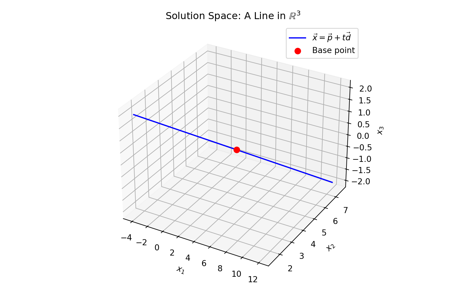
Reward: Parametric vector form gives full insight into the structure of the solution set for the underlying system. The ability to interpret the solution set geometrically, as a line in this case, gives us greater understanding of the solution vectors.
Free Variables and the Geometry of Solution Spaces
As in our example, the number of free variables determines the shape of the solution space. Each free variable corresponds to a directional vector that solutions can travel along.
- The solution space for a system with no free variables is a single point.
- The solution space for a system with exactly one free variable is a line.
- The solution space for a system with exactly two free variables is a plane.
- The solution space for a system with three or more free variables is a hyperplane.
Examples to Try #1
Write the corresponding matrix equation and the augmented coefficient matrix. Transform the matrix into its equivalent reduced row echelon form and identify the pivot columns and highlight any free variables. Write the solution of the system in parametric vector form and describe the geometry of the solution space.
- \(\left\{\begin{array}{rcr} x_1 + 2x_2 - x_3 & = & 4\\ 2x_1 + x_2 + x_3 & = & 7\\ -3x_1 + 4x_2 + 2x_3 & = & -1\end{array}\right.\)
Examples to Try #2
Write the corresponding matrix equation and the augmented coefficient matrix. Transform the matrix into its equivalent reduced row echelon form and identify the pivot columns and highlight any free variables. Write the solution of the system in parametric vector form and describe the geometry of the solution space.
- \(\left\{\begin{array}{rcr} x_1 - 2x_2 + 3x_3 & = & 1\\ 2x_1 + x_2 - x_3 & = & 4\end{array}\right.\)
Examples to Try #3
Write the corresponding matrix equation and the augmented coefficient matrix. Transform the matrix into its equivalent reduced row echelon form and identify the pivot columns and highlight any free variables. Write the solution of the system in parametric vector form and describe the geometry of the solution space.
- \(\left\{\begin{array}{rcr} x_1 + x_2 + x_3 & = & 3\\ 2x_1 + 3x_2 + 4x_3 & = & 8\\ -3x_1 - 2x_2 - x_3 & = & -5\\ x_1 + 2x_2 + 3x_3 & = & 6\end{array}\right.\)
Examples to Try #4
Write the corresponding matrix equation and the augmented coefficient matrix. Transform the matrix into its equivalent reduced row echelon form and identify the pivot columns and highlight any free variables. Write the solution of the system in parametric vector form and describe the geometry of the solution space.
- \(\left\{\begin{array}{rcr} x_1 + x_2 & = & 2\\ 2x_1 - x_2 & = & 1\\ 3x_1 + x_2 & = & 5\end{array}\right.\)
Examples to Try #5
Write the corresponding matrix equation and the augmented coefficient matrix. Transform the matrix into its equivalent reduced row echelon form and identify the pivot columns and highlight any free variables. Write the solution of the system in parametric vector form and describe the geometry of the solution space.
- \(\left\{\begin{array}{rcr} x_1 + 2x_2 - x_3 + x_4 & = & 0\\ 2x_1 - x_2 + 3x_3 - x_4 & = & 5\end{array}\right.\)
Homework
\[\Huge{\text{Start Homework 3}}\] \[\Huge{\text{on MyOpenMath}}\]
Next Time…
\(\Huge{\text{Row Reduction Workshop}}\)