MAT 350: Determinants
November 10, 2025
Warm-Up Problems
Complete the following warm-up problems to re-familiarize yourself with concepts we’ll be leveraging today.
Consider the standard basis vectors for \(\mathbb{R}^2\), \(\vec{v_1} = \begin{bmatrix} 1\\ 0\end{bmatrix}\) and \(\vec{v_2} = \begin{bmatrix} 0\\ 1\end{bmatrix}\).
- Draw the vectors \(\vec{v_1}\), \(\vec{v_2}\), and \(\vec{v_1} + \vec{v_2}\).
- Calculate the area of the shape enclosed by these vectors.
- Consider the matrix \(A = \begin{bmatrix} 2 & 0\\ 0 & 3\end{bmatrix}\). Calculate \(A\vec{v_1}\) and \(A\vec{v_2}\).
- Draw the vectors \(A\vec{v_1}\), \(A\vec{v_2}\), and \(A\vec{v_1} + A\vec{v_2}\).
- Calculate the area enclosed within this new shape. Can you connect the change in area to the structure of the matrix \(A\)?
Reminders and Today’s Goal
Vectors are elements of a space (\(\mathbb{R}^n\), for example), with both direction and magnitude.
Vectors are added head to tail
- If \(\vec{v_1}\) and \(\vec{v_2}\) are linearly independent (non-parallel) in \(\mathbb{R}^2\), then the vectors \(\vec{v_1}\), \(\vec{v_2}\), and \(\vec{v_1} + \vec{v_2}\) form the vertices of a parallelogram
- If \(\vec{v_1}\), \(\vec{v_2}\), and \(\vec{v_3}\) are linearly independent vectors in \(\mathbb{R}^3\), then the vectors along with the sums \(\vec{v_1} + \vec{v_2}\), \(\vec{v_1} + \vec{v_3}\), and \(\vec{v_2} + \vec{v_3}\) form the vertices of a parallelepiped.
We say that a matrix with \(m\) rows and \(n\) columns is an \(m\times n\) matrix – if a matrix has the same number of rows and columns, we call it square.
We can view square matrices as functions that transform vectors (or shapes) in their space (\(\mathbb{R}^n\)).
Reminders and Today’s Goal
Goals for Today: After today’s discussion, you should be able to
- Provide geometric interpretations of the determinant.
- Identify conclusions that can be made about a matrix and its columns when a determinant is \(0\).
- Calculate the determinant of a \(2\times 2\) matrix.
- Use strategic cofactor expansions to calculate the determinant of \(3\times 3\) or larger matrices.
- Quickly calculate the determinant of triangular matrices, and identify the utility of conducting row-reduction before calculating a determinant.
Motivation for Determinants
A parallelogram created using the vectors \(\vec{v_1} = \begin{bmatrix} 1\\ 0\end{bmatrix}\) and \(\vec{v_2} = \begin{bmatrix} 0\\ 1\end{bmatrix}\)
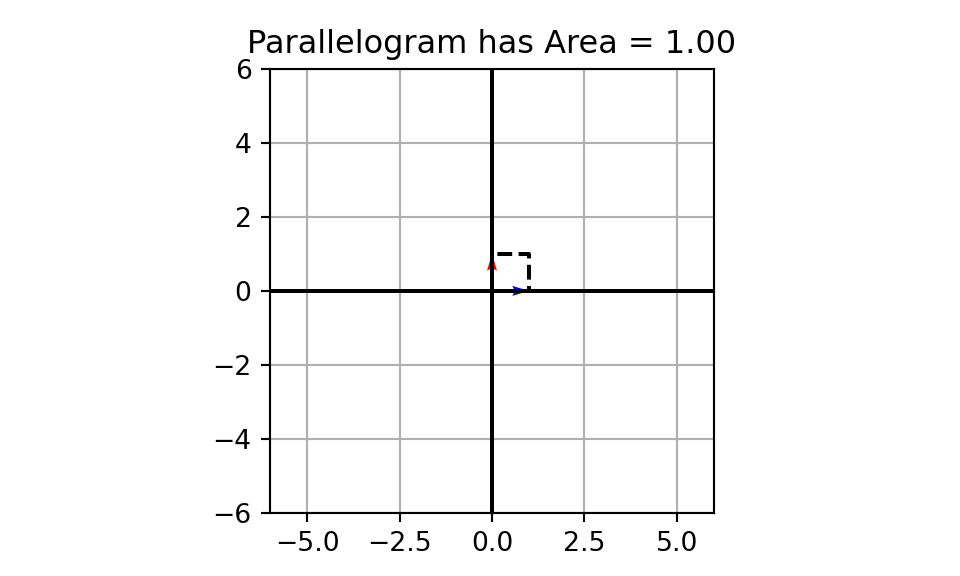
Motivation for Determinants
A parallelogram created using the vectors \(\vec{v_1} = \begin{bmatrix} 1\\ 0\end{bmatrix}\) and \(\vec{v_2} = \begin{bmatrix} 0\\ 1\end{bmatrix}\)

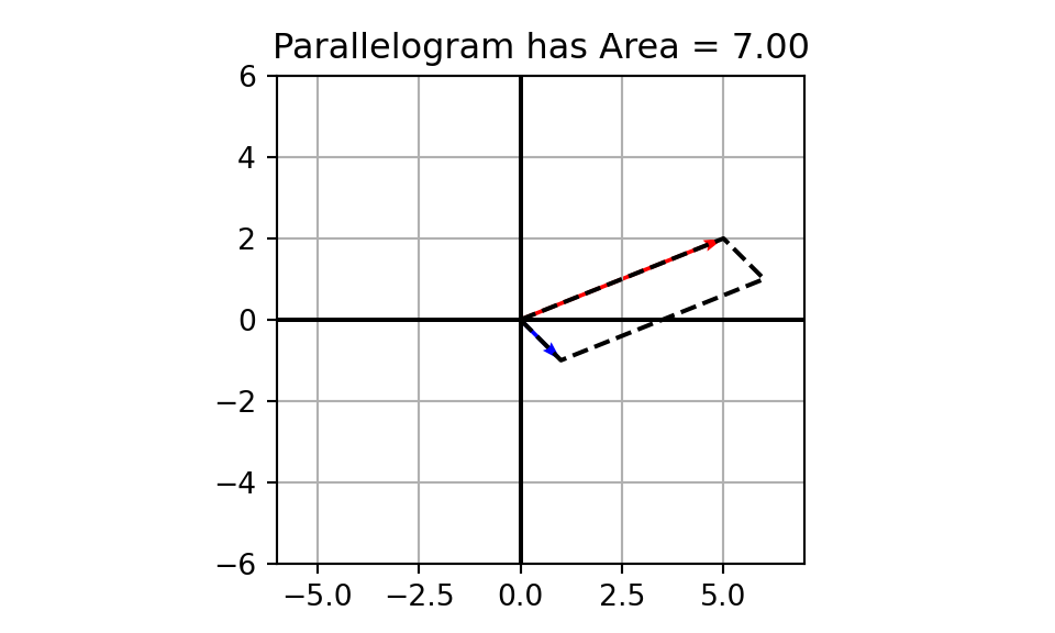
A parallelogram created using the vectors \(\vec{u_1} = \begin{bmatrix} 5\\ 2\end{bmatrix}\) and \(\vec{u_2} = \begin{bmatrix} 1\\ -1\end{bmatrix}\)
Check out this interactive parallelogram explorer and experiment with different initial vectors in both the \(\mathbb{R}^2\) and \(\mathbb{R}^3\) settings.
Explore a variety of vectors including linearly independent and linearly dependent sets.
Summary of Takeaways
Think about what you observed as you explored different combinations of initial vectors in both the \(\mathbb{R}^2\) and \(\mathbb{R}^3\) settings.
Summary: The area of a parallelogram formed by two two-dimensional vectors, the volume of a parallelepiped formed by three three-dimensional vectors, and their higher dimensional analogs can be used to identify whether or not…
- the columns of a matrix are linearly independent
- the matrix is invertible
If the column vectors are not linearly independent, then the dimension of the shape formed by those column vectors collapses and the corresponding measure (area, volume, etc.) will be \(0\).
In this case, the matrix is not invertible.
The Determinant for Area, Volume, and Higher-Dimensional Analogs
We’ve identified that the area, volume, etc. will give us information about the invertibility of a matrix.
Claim (without proof): Determinants will calculate these quantities for us.
- One caveat though is that it is possible to have a negative determinant.
- This is the case if pairs of vectors are negatively oriented, meaning that the angle measured counterclockwise between consecutive column vectors \(\vec{v_i}\) and \(\vec{v_{i+1}}\) is greater than \(180^\circ\).
Calculating Determinants
We saw the definition of a determinant of a \(2\times 2\) matrix during our discussion on invertibility.
Recall (Inverse of a \(2\times 2\) Matrix): Let \(A = \left[\begin{array}{rr} a & b\\ c & d\end{array}\right]\), then as long as \(\det\left(A\right) = ad - bc\) is non-zero, we have that \(A\) is invertible and \(\displaystyle{A^{-1} = \frac{1}{ad - bc}\left[\begin{array}{rr} d & -b\\ -c & a\end{array}\right]}\).
We’ll add to this by showing how to compute the determinant of a square matrix which is larger than \(2\times 2\), but for now, the definition of the determinant of a \(2\times 2\) matrix is reiterated below.
Definition (Determinant of a \(2\times 2\) Matrix): Consider the matrix \(A = \left[\begin{array}{rr} a & b\\ c & d\end{array}\right]\). We have \(\det\left(A\right) = ad - bc\).
Completed Example #1
Definition (Determinant of a \(2\times 2\) Matrix): Consider the matrix \(A = \left[\begin{array}{rr} a & b\\ c & d\end{array}\right]\). We have \(\det\left(A\right) = ad - bc\).
Example: Find the determinant of the matrix \(A = \left[\begin{array}{rr} 2 & -6\\ 1 & 5\end{array}\right]\).
\[\begin{align*} \det\left(\left[\begin{array}{rr} 2 & -6\\ 1 & 5\end{array}\right]\right) \end{align*}\]
Completed Example #1
Definition (Determinant of a \(2\times 2\) Matrix): Consider the matrix \(A = \left[\begin{array}{rr} a & b\\ c & d\end{array}\right]\). We have \(\det\left(A\right) = ad - bc\).
Example: Find the determinant of the matrix \(A = \left[\begin{array}{rr} 2 & -6\\ 1 & 5\end{array}\right]\).
\[\begin{align*} \det\left(\left[\begin{array}{rr} 2 & -6\\ 1 & 5\end{array}\right]\right) &= 2\left(5\right) - \left(-6\right)\left(1\right) \end{align*}\]
Completed Example #1
Definition (Determinant of a \(2\times 2\) Matrix): Consider the matrix \(A = \left[\begin{array}{rr} a & b\\ c & d\end{array}\right]\). We have \(\det\left(A\right) = ad - bc\).
Example: Find the determinant of the matrix \(A = \left[\begin{array}{rr} 2 & -6\\ 1 & 5\end{array}\right]\).
\[\begin{align*} \det\left(\left[\begin{array}{rr} 2 & -6\\ 1 & 5\end{array}\right]\right) &= 2\left(5\right) - \left(-6\right)\left(1\right)\\ &= 10 + 6 \end{align*}\]
Completed Example #1
Definition (Determinant of a \(2\times 2\) Matrix): Consider the matrix \(A = \left[\begin{array}{rr} a & b\\ c & d\end{array}\right]\). We have \(\det\left(A\right) = ad - bc\).
Example: Find the determinant of the matrix \(A = \left[\begin{array}{rr} 2 & -6\\ 1 & 5\end{array}\right]\).
\[\begin{align*} \det\left(\left[\begin{array}{rr} 2 & -6\\ 1 & 5\end{array}\right]\right) &= 2\left(5\right) - \left(-6\right)\left(1\right)\\ &= 10 + 6\\ &= 16 \end{align*}\]
Interpretations: The area of the parallelogram created by the vectors \(\vec{v_1} = \begin{bmatrix} 2\\ 1\end{bmatrix}\) and \(\vec{v_2} = \begin{bmatrix} -6\\ 5\end{bmatrix}\) is \(16\), and the matrix \(A\) is invertible.
Examples to Try #1
Definition (Determinant of a \(2\times 2\) Matrix): Consider the matrix \(A = \left[\begin{array}{rr} a & b\\ c & d\end{array}\right]\). We have \(\det\left(A\right) = ad - bc\).
Example: Calculate the determinant of each of the following \(2\times 2\) matrices.
- \(A = \begin{bmatrix} 5 & 1\\ 2 & 6\end{bmatrix}\)
- \(B = \begin{bmatrix} 6 & 2\\ 18 & 6\end{bmatrix}\)
- \(C = \begin{bmatrix} 2 & 7\\ 3 & 9\end{bmatrix}\)
Cofactor Expansion for Larger Matrices
Definition (\(ij\)-Cofactor of \(A\)): Let \(A\) be an \(n\times n\) matrix. We define the \(ij\)-cofactor of \(A\), denoted by \(A_{ij}\) to be the \(\left(n-1\right) \times \left(n-1\right)\) matrix obtained from \(A\) by deleting row i and column j.
Definition (Determinant of an \(n\times n\) Matrix): Let \(A\) be an \(n\times n\) matrix. We can compute \(\det\left(A\right)\) using cofactor expansion along any row, \(i\). That is,
\[\begin{align*}\det\left(A\right) &= \sum_{j = 1}^{n}{\left(-1\right)^{i+j}a_{ij}\det\left(A_{ij}\right)}\\ &= \left(-1\right)^{i + 1}a_{i1}\det\left(A_{i1}\right) + \left(-1\right)^{i + 2}a_{i2}\det\left(A_{i2}\right) + \cdots + \left(-1\right)^{i + n}a_{in}\det\left(A_{in}\right) \end{align*}\]
- The above definition is recursive.
- That is, if \(A_{ij}\) is not a \(2\times 2\) matrix, we can use cofactor expansion to determine the determinant of \(A_{ij}\).
Completed Example #2
Example Compute the determinant of the matrix \(A = \left[\begin{array}{rrr} 1 & -2 & 5\\ 0 & 4 & 1\\ 1 & 2 & -1\end{array}\right]\).
\[\begin{align*} \det\left(\left[\begin{array}{rrr} 1 & -2 & 5\\ 0 & 4 & 1\\ 1 & 2 & -1\end{array}\right]\right) \end{align*}\]
Completed Example #2
Example Compute the determinant of the matrix \(A = \left[\begin{array}{rrr} 1 & -2 & 5\\ 0 & 4 & 1\\ 1 & 2 & -1\end{array}\right]\).
\[\begin{align*} \det\left(\left[\begin{array}{rrr} 1 & -2 & 5\\ 0 & 4 & 1\\ 1 & 2 & -1\end{array}\right]\right) &= 1\det\left(\left[\begin{array}{rr} 4 & 1\\ 2 & -1\end{array}\right]\right) - \left(-2\right)\det\left(\left[\begin{array}{rr} 0 & 1\\ 1 & -1\end{array}\right]\right) + 5\det\left(\left[\begin{array}{rr} 0 & 4\\ 1 & 2\end{array}\right]\right) \end{align*}\]
Completed Example #2
Example Compute the determinant of the matrix \(A = \left[\begin{array}{rrr} 1 & -2 & 5\\ 0 & 4 & 1\\ 1 & 2 & -1\end{array}\right]\).
\[\begin{align*} \det\left(\left[\begin{array}{rrr} 1 & -2 & 5\\ 0 & 4 & 1\\ 1 & 2 & -1\end{array}\right]\right) &= 1\det\left(\left[\begin{array}{rr} 4 & 1\\ 2 & -1\end{array}\right]\right) - \left(-2\right)\det\left(\left[\begin{array}{rr} 0 & 1\\ 1 & -1\end{array}\right]\right) + 5\det\left(\left[\begin{array}{rr} 0 & 4\\ 1 & 2\end{array}\right]\right)\\ &= \left(4\left(-1\right) - 1\left(2\right)\right) + 2\left(0\left(-1\right) - 1\left(1\right)\right) + 5\left(0\left(2\right) - 4\left(1\right)\right)\\ \end{align*}\]
Completed Example #2
Example Compute the determinant of the matrix \(A = \left[\begin{array}{rrr} 1 & -2 & 5\\ 0 & 4 & 1\\ 1 & 2 & -1\end{array}\right]\).
\[\begin{align*} \det\left(\left[\begin{array}{rrr} 1 & -2 & 5\\ 0 & 4 & 1\\ 1 & 2 & -1\end{array}\right]\right) &= 1\det\left(\left[\begin{array}{rr} 4 & 1\\ 2 & -1\end{array}\right]\right) - \left(-2\right)\det\left(\left[\begin{array}{rr} 0 & 1\\ 1 & -1\end{array}\right]\right) + 5\det\left(\left[\begin{array}{rr} 0 & 4\\ 1 & 2\end{array}\right]\right)\\ &= \left(4\left(-1\right) - 1\left(2\right)\right) + 2\left(0\left(-1\right) - 1\left(1\right)\right) + 5\left(0\left(2\right) - 4\left(1\right)\right)\\ &= -6 - 2 - 20\\ \end{align*}\]
Completed Example #2
Example Compute the determinant of the matrix \(A = \left[\begin{array}{rrr} 1 & -2 & 5\\ 0 & 4 & 1\\ 1 & 2 & -1\end{array}\right]\).
\[\begin{align*} \det\left(\left[\begin{array}{rrr} 1 & -2 & 5\\ 0 & 4 & 1\\ 1 & 2 & -1\end{array}\right]\right) &= 1\det\left(\left[\begin{array}{rr} 4 & 1\\ 2 & -1\end{array}\right]\right) - \left(-2\right)\det\left(\left[\begin{array}{rr} 0 & 1\\ 1 & -1\end{array}\right]\right) + 5\det\left(\left[\begin{array}{rr} 0 & 4\\ 1 & 2\end{array}\right]\right)\\ &= \left(4\left(-1\right) - 1\left(2\right)\right) + 2\left(0\left(-1\right) - 1\left(1\right)\right) + 5\left(0\left(2\right) - 4\left(1\right)\right)\\ &= -6 - 2 - 20\\ &= -28 \end{align*}\]
Note. We could have saved a bit of work by expanding along the first column or the second row, taking advantage of the \(0\) element in the matrix. We would end up with the same determinant – we just need to take care in determining the signs on the terms in the cofactor expansion.
Example to Try #2
Example Compute the determinant of the matrix \(A = \left[\begin{array}{rrr} 1 & -2 & 5\\ 0 & 4 & 1\\ 1 & 2 & -1\end{array}\right]\) by using cofactor expansion along the second row instead of the first
Example Compute the determinant of the matrix \(A = \left[\begin{array}{rrr} 0 & 1 & 7\\ -2 & 1 & 8\\ 0 & -9 & -2\end{array}\right]\).
Limitations to Cofactor Expansion
Note (Feasibility of Computing Determinants): At the beginning of our semester, we discussed that linear systems modeling real-world systems could easily utilize hundreds or thousands of variables and have hundreds or thousands of constraint equations.
Even considering a \(25\times 25\) matrix, a computer performing a trillion multiplications per second would take half a million years to compute its determinant using cofactor expansion!
Algorithmic Complexity of Cofactor Expansion: The complexity of cofactor expansion to compute a determinant is on the order of \(n!\). Computer scientists would say that the algorithm is \(O\left(n!\right)\) – which is very bad!
Fortunately there are faster methods, some of which exploit the structure of a matrix. One of those methods appears below.
Determinants of Triangular Matrices
Definition (Triangular Matrix): A matrix \(A\) having all entries either above or below its main diagonal as \(0\)’s is called a triangular matrix. If the \(0\)’s are below the main diagonal, \(A\) is called lower triangular while a matrix having all \(0\)’s above the main diagonal is upper triangular.
\[A = \begin{bmatrix} 2 & 8 & -3\\ 0 & 7 & 9\\ 0 & 0 & -1\end{bmatrix}~~~~~~B = \begin{bmatrix} 6 & 0 & 0 & 0\\ -2 & 0 & 0 & 0\\ -1 & 3 & 1 & 0\\ 2 & 0 & -7 & 5\end{bmatrix}\]
Strategy (Determinants of Triangular Matrices): If \(A\) is a triangular matrix, then \(\det\left(A\right)\) is the product of the entries along the main diagonal of \(A\).
Great News! We can convert any square matrix into a triangular matrix using row-reduction, which only has complexity \(O\left(n^3\right)\) – an enormous improvement.
Completed Example #3
Example: Find the determinant of the matrix \(A = \left[\begin{array}{rrrr} 2 & 1 & -4 & 8\\ 0 & -1 & 8 & 3\\ 0 & 0 & -3 & 0\\ 0 & 0 & 0 & 4\end{array}\right]\).
Since the matrix is an upper-triangular matrix, its determinant is the product of its diagonal elements.
That is, \(\det\left(A\right) = 2\left(-1\right)\left(-3\right)\left(4\right) = 24\).
Interpretations: The volume of the parallelepiped bounded by the column vectors of \(A\) is \(24\). Additionally, the matrix \(A\) is invertible!
Example to Try #3
Example: Calculate the determinants of each of the following triangular matrices. Interpret the determinants in terms of areas or volumes and discuss what the determinant reveals about invertibility.
\[A = \begin{bmatrix} 2 & 8 & -3\\ 0 & 7 & 9\\ 0 & 0 & -1\end{bmatrix}~~~~~~B = \begin{bmatrix} 6 & 0 & 0 & 0\\ -2 & 0 & 0 & 0\\ -1 & 3 & 1 & 0\\ 2 & 0 & -7 & 5\end{bmatrix}\]
Computing Determinants with Python
As with several other topics from this course, we can utilize a computing environment to help us with calculations.
As mentioned previously, cofactor expansion is a slow procedure so, “under the hood”, Python will make use of alternative strategies that exploit or change matrix structure.
{sympy}
{numpy}
Computing Determinants with Python
As with several other topics from this course, we can utilize a computing environment to help us with calculations.
As mentioned previously, cofactor expansion is a slow procedure so, “under the hood”, Python will make use of alternative strategies that exploit or change matrix structure.
Remember. With {numpy} we must explicitly indicate that our matrix elements should be considered as floats rather than integers.
Alternative Notation
Before moving to examples for you to try, it is useful to mention some common notation.
When stating that we are computing the determinant of a matrix, it is common to replace the brackets on either end of the matrix by vertical bars.
For example, instead of writing \(\det\left(\left[\begin{array}{rrr} a & b & c\\ d & e & f\\ g & h & i\end{array}\right]\right)\), it is common to write \(\left|\begin{array}{rrr} a & b & c\\ d & e & f\\ g & h & i\end{array}\right|\) instead.
Examples to Try (1 of 3)
- Use the fact that if \(A = \left[\begin{array}{rr} a & b\\ c & d\end{array}\right]\), then \(\det\left(A\right) = ad - bc\) to compute the determinants of the following \(2\times 2\) matrices.
\[A = \left[\begin{array}{rr} 2 & 6\\ -3 & 5\end{array}\right] ~~~~~~~ B = \left[\begin{array}{rr} -1 & 3\\ 8 & 2\end{array}\right]\]
- Use cofactor expansion to compute the determinants of the following \(3\times 3\) matrices.
\[A = \left[\begin{array}{rrr} 1 & 2 & -1\\ -3 & 0 & 5\\ 4 & 2 & -1\end{array}\right] ~~~~~ B = \left[\begin{array}{rrr} 2 & -5 & 4\\ 0 & 1 & 0\\ 1 & 1 & 1\end{array}\right] ~~~~~ C = \left[\begin{array}{rrr} 3 & -1 & -1\\ 1 & 2 & 4\\ -3 & -1 & -2\end{array}\right]\]
More Examples to Try (2 of 3)
- Compute the determinants of the following triangular matrices.
\[A = \left[\begin{array}{rr} 2 & 9\\ 0 & 3\end{array}\right] ~~~~~ B = \left[\begin{array}{rrr} -1 & 0 & 0 \\ 2 & 3 & 0\\ 3 & -3 & -5\end{array}\right] ~~~~~ C = \left[\begin{array}{rrrrr} 2 & 0 & 1 & 8 & 1\\ 0 & 1 & 0 & 0 & 0\\ 0 & 0 & 4 & 8 & -2\\ 0 & 0 & 0 & 3 & -1\\ 0 & 0 & 0 & 0 & 2\end{array}\right]\]
- Use strategic choices about cofactor expansion to compute the determinants of the following matrices.
\[A = \left[\begin{array}{rrrr} 1 & 2 & -5 & 1\\ -3 & 1 & 8 & 1\\ 0 & 2 & 0 & 0\\ 0 & -1 & 0 & 1\end{array}\right] ~~~~~~ B = \left[\begin{array}{rrrrr} 2 & -1 & 3 & 6 & 2\\ 0 & 0 & 5 & 0 & 0\\ 0 & -3 & 1 & 4 & -2\\ 0 & 0 & 2 & 1 & 7\\ 0 & 0 & 3 & 0 & 2\end{array}\right]\]
General Examples to Try (3 of 3)
Determine the impact of a row-swap operation on a \(2\times 2\) matrix by finding \(\det\left(\left[\begin{array}{rr} a & b\\ c & d\end{array}\right]\right)\) and \(\det\left(\left[\begin{array}{rr} c & d\\ a & b\end{array}\right]\right)\).
Determine the impact of scaling a row of a \(2\times 2\) matrix by a constant \(k\) by comparing \(\det\left(\left[\begin{array}{rr} a & b\\ kc & kd\end{array}\right]\right)\) to \(\det\left(\left[\begin{array}{rr} a & b\\ c & d\end{array}\right]\right)\).
Determine the impact on the determinant of a \(2\times 2\) matrix if we add a scalar multiple of the second row to the first row by comparing \(\det\left(\left[\begin{array}{rr} a + kc & b + kd\\ b & c\end{array}\right]\right)\) to \(\det\left(\left[\begin{array}{rr} a & b\\ b & c\end{array}\right]\right)\).
Exit Ticket Task
Navigate to our MAT350 Exit Ticket Form, answer the questions, and complete the task below.
Note. Today’s discussion is listed as 17. Determinants
Task: Find the determinant of the \(3\times 3\) matrix below, determine what that means geometrically about the column vectors, the corresponding linear transformation, and the matrix itself.
\[A = \begin{bmatrix} 3 & 0 & -6\\ -1 & 5 & 7\\ -4 & 0 & 8\end{bmatrix}\]
Homework
\[\Huge{\text{Complete Homework 9}}\] \[\Huge{\text{on MyOpenMath}}\]
Next Time…
\(\Huge{\text{Subspaces}}\)
Comments on Cofactor Expansion
Definition (Determinant of an \(n\times n\) Matrix): Let \(A\) be an \(n\times n\) matrix. We can compute \(\det\left(A\right)\) using cofactor expansion along any row, \(i\). That is,
\[\begin{align*}\det\left(A\right) &= \sum_{j = 1}^{n}{\left(-1\right)^{i+j}a_{ij}\det\left(A_{ij}\right)}\\ &= \left(-1\right)^{i + 1}a_{i1}\det\left(A_{i1}\right) + \left(-1\right)^{i + 2}a_{i2}\det\left(A_{i2}\right) + \cdots + \left(-1\right)^{i + n}a_{in}\det\left(A_{in}\right) \end{align*}\]
Computing the determinant of a large matrix requires good organization and book-keeping.
In order to get comfortable with the process of computing determinants, we’ll compute determinants of \(2\times 2\), \(3\times 3\), and some \(4\times 4\) matrices by hand.
We’ll also compute the determinants of larger matrices by hand if they have convenient structure.