Inference on Population Means
Single Populations and Comparisons Between Two Groups
January 3, 2026
Highlights
Reminders on statistical inference
Additional uncertainty with inference on means
The \(t\)-distributions
- Calculating probabilities (useful for obtaining \(p\)-values)
- Identifying quantiles (useful for finding critical values for confidence intervals)
Examples
- One Sample Hypothesis Testing Completed Example
- Two Sample Hypothesis Testing Example Together
- One Sample Confidence Interval Example Together
- Two Sample Confidence Interval Completed Example
- Mixed Examples
Reminders on Inference and Inferential Tools
We use statistical inference to make or test claims about population parameters which we cannot measure directly
- We make claims by constructing confidence intervals
- We test claims by conducting hypothesis tests
Confidence intervals provide a range of plausible values for a population parameter
\[\left(\begin{array}{c}\text{point}\\ \text{estimate}\end{array}\right) \pm \left(\begin{array}{c}\text{critical}\\ \text{value}\end{array}\right)\left(\begin{array}{c}\text{standard}\\ \text{error}\end{array}\right)\]
Hypothesis tests provide a framework for testing claims about a population parameter, with major steps including…
- Read the scenario
- Write out the two hypotheses
- Draw a picture
- Declare the level of significance
- Calculate a test statistic
- Convert it into a \(p\)-value
- Compare the \(p\)-value to \(\alpha\)
- Interpret the results in context
Where We Are; Where We’re Going…
| Inference On... | "Test" Name |
|---|---|
| One Binary Categorical Variable | One Sample z |
| Association Between Two Binary Categorical Variables | Two Sample z |
| One MultiClass Categorical Variable | Chi-Squared GOF |
| Associations Between Two MultiClass Categorical Variables | Chi-Squared Independence |
Where We Are; Where We’re Going
| Inference On... | "Test" Name |
|---|---|
| One Binary Categorical Variable | One Sample z |
| Association Between Two Binary Categorical Variables | Two Sample z |
| One MultiClass Categorical Variable | Chi-Squared GOF |
| Associations Between Two MultiClass Categorical Variables | Chi-Squared Independence |
| One Numerical Variable | One Sample t |
| Association Between a Numerical Variable and a Binary Categorical Variable | Two Sample t |
| Association Between a Numerical Variable and a MultiClass Categorical Variable | |
| Association Between a Numerical Variable and a Single Other Numerical Variable | |
| Association Between a Numerical Variable and Many Other Variables | |
| Association Between a Categorical Variable and Many Other Variables | ✘ |
Additional Uncertainty with Means
When doing inference, we utilize the sampling distribution
With categorical data, our sampling distribution has a mean and standard error which depend only on a single parameter – the population proportion(s) \(p\)/\(p_1\)/\(p_2\)
For numerical data, the mean of the sampling distribution is the population mean \(\mu\) and the standard error given by \(\sigma/\sqrt{n}\)
With means, we have additional uncertainty associated with estimating the sampling distribution because we are approximating more population parameters via our sample data
Because of this additional uncertainty, using the normal distribution is too optimistic and we use a “penalized” distribution instead
The \(t\)-distributions
The distribution we use to account for additional uncertainty is a \(t\)-distribution, from a family of distributions
These distributions were first used by a brewmaster at Guinness who was trying to estimate alcohol content of beer using small samples
These distributions have “heavier tails” than the normal distribution, reflecting greater variability when using a sample standard deviation \(s\) to estimate the population standard deviation \(\sigma\)
As sample size grows, the \(t\)-distribution becomes closer to the normal distribution, since more data provides a more stable estimate of \(\sigma\)
Each \(t\)-distribution is characterized by its degrees of freedom (\(\texttt{df}\)), which typically equals \(n - 1\) for a single sample
This accounts for the number of observations in our sample that are free to vary after using one value to estimate the mean
Calculating Probability
- Find the probability of observing a value to the left of -1.96 on a \(t\)-distribution with 11 degrees of freedom.

Calculating Probability
- Find the probability of observing a value to the left of -1.96 on a \(t\)-distribution with 11 degrees of freedom.

pt(-1.96, df = 11) \(\approx\) 0.0379072
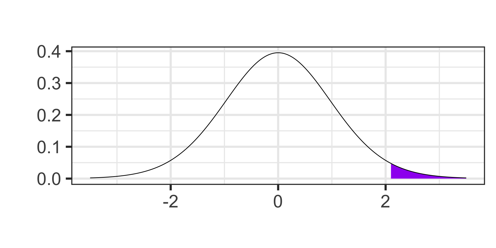
- Find the probability of observing a value to the right of 2.1 on a \(t\)-distribution with 26 degrees of freedom.
Calculating Probability
- Find the probability of observing a value to the left of -1.96 on a \(t\)-distribution with 11 degrees of freedom.
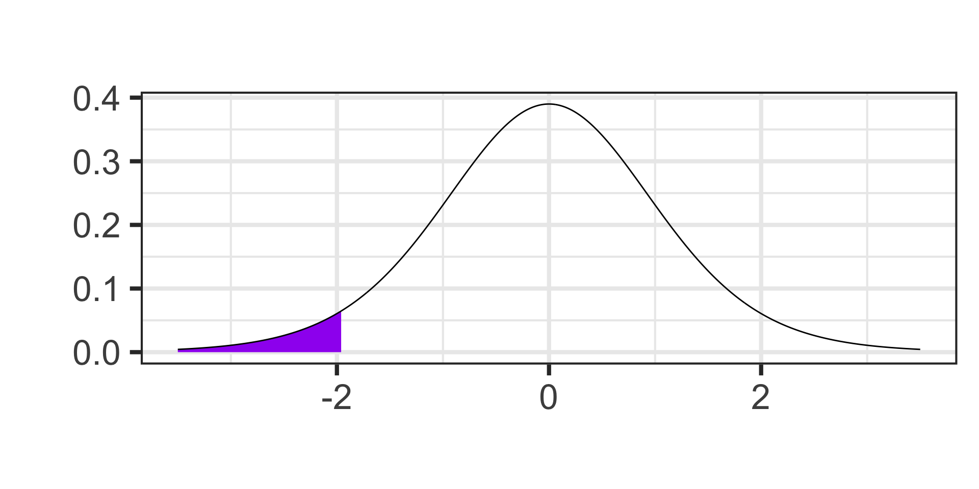
pt(-1.96, df = 11) \(\approx\) 0.0379072
- Find the probability of observing a value to the right of 2.1 on a \(t\)-distribution with 26 degrees of freedom.
1 - pt(2.1, df = 26) \(\approx\) 0.0227907

Identifying Quantiles
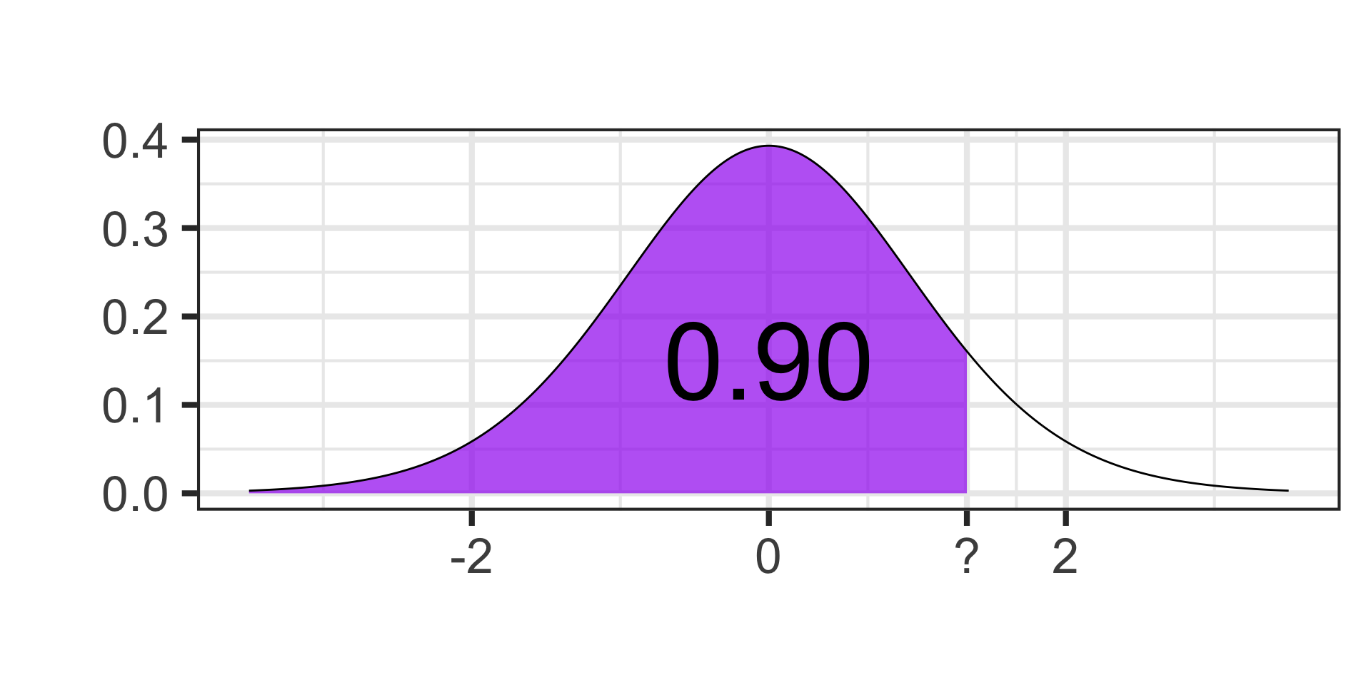
- Find the cutoff value on a \(t\)-distribution with 17 degrees of freedom for which 90% of the area falls below.

Identifying Quantiles
- Find the cutoff value on a \(t\)-distribution with 17 degrees of freedom for which 90% of the area falls below.
qt(0.90, df = 17) \(\approx\) 1.33

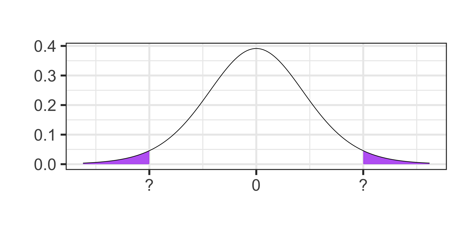
- Find the critical value for a 95% confidence interval on a \(t\)-distribution with 13 degrees of freedom.

Identifying Quantiles
- Find the cutoff value on a \(t\)-distribution with 17 degrees of freedom for which 90% of the area falls below.
qt(0.90, df = 17) \(\approx\) 1.33
- Find the critical value for a 95% confidence interval on a \(t\)-distribution with 13 degrees of freedom.

Each tail contains half of the 5% of area that remains
Identifying Quantiles
- Find the cutoff value on a \(t\)-distribution with 17 degrees of freedom for which 90% of the area falls below.
qt(0.90, df = 17) \(\approx\) 1.33

- Find the critical value for a 95% confidence interval on a \(t\)-distribution with 13 degrees of freedom.

Each tail contains 2.5% of the area
Identifying Quantiles
- Find the cutoff value on a \(t\)-distribution with 17 degrees of freedom for which 90% of the area falls below.
qt(0.90, df = 17) \(\approx\) 1.33

- Find the critical value for a 95% confidence interval on a \(t\)-distribution with 13 degrees of freedom.
Each tail contains 2.5% of the area
qt(1 - 0.025, df = 13) \(\approx\) 2.16
Hypothesis Test for a Population Mean
Scenario: A car manufacturer claims that the average annual repair cost for their new model is no more than $400. To validate this claim, a consumer group gathers a sample of 30 car owners and finds an average annual repair cost of $450 with a standard deviation of $150. Does this sample provide evidence that the car manufacturer’s claim is incorrect?
- \(\begin{array}{lcl} H_0 & : & \mu = 400\\ H_a & : & \mu > 400\end{array}\)
- Samples satisfying \(H_a\) are

- \(\alpha = 0.05\)
- \(S_E = ?\)
Hypothesis Test for a Population Mean
Scenario: A car manufacturer claims that the average annual repair cost for their new model is no more than $400. To validate this claim, a consumer group gathers a sample of 30 car owners and finds an average annual repair cost of $450 with a standard deviation of $150. Does this sample provide evidence that the car manufacturer’s claim is incorrect?
- \(\begin{array}{lcl} H_0 & : & \mu = 400\\ H_a & : & \mu > 400\end{array}\)
- Samples satisfying \(H_a\) are
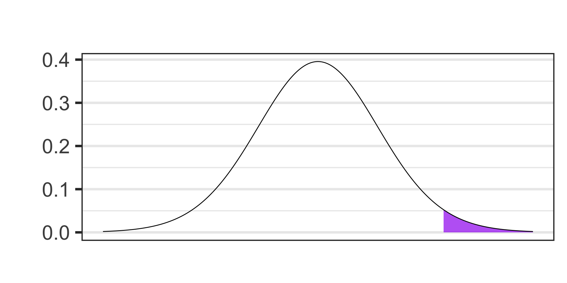
- \(\alpha = 0.05\)
- \(S_E = s/\sqrt{n},~~~\text{df} = n - 1\)
Hypothesis Test for a Population Mean
Scenario: A car manufacturer claims that the average annual repair cost for their new model is no more than $400. To validate this claim, a consumer group gathers a sample of 30 car owners and finds an average annual repair cost of $450 with a standard deviation of $150. Does this sample provide evidence that the car manufacturer’s claim is incorrect?
- \(\begin{array}{lcl} H_0 & : & \mu = 400\\ H_a & : & \mu > 400\end{array}\)
- Samples satisfying \(H_a\) are

- \(\alpha = 0.05\)
- \(S_E = s/\sqrt{n} = \frac{150}{\sqrt{30}} \approx 27.39,~~~\text{df} = n - 1\)
- \(\displaystyle{t = \frac{\left(\text{point est.}\right) - \left(\text{null val.}\right)}{S_E}}\)
Hypothesis Test for a Population Mean
Scenario: A car manufacturer claims that the average annual repair cost for their new model is no more than $400. To validate this claim, a consumer group gathers a sample of 30 car owners and finds an average annual repair cost of $450 with a standard deviation of $150. Does this sample provide evidence that the car manufacturer’s claim is incorrect?
- \(\begin{array}{lcl} H_0 & : & \mu = 400\\ H_a & : & \mu > 400\end{array}\)
- Samples satisfying \(H_a\) are

- \(\alpha = 0.05\)
- \(S_E = s/\sqrt{n} \approx 27.39,~~~\text{df} = n - 1\)
- \(t = \frac{450 - 400}{27.39} \approx 1.83\)
- \(p\)-value…
Hypothesis Test for a Population Mean
Scenario: A car manufacturer claims that the average annual repair cost for their new model is no more than $400. To validate this claim, a consumer group gathers a sample of 30 car owners and finds an average annual repair cost of $450 with a standard deviation of $150. Does this sample provide evidence that the car manufacturer’s claim is incorrect?
- \(\begin{array}{lcl} H_0 & : & \mu = 400\\ H_a & : & \mu > 400\end{array}\)
- Samples satisfying \(H_a\) are

- \(\alpha = 0.05\)
- \(S_E = s/\sqrt{n} \approx 27.39,~~~\text{df} = n - 1\)
- \(t = \frac{450 - 400}{27.39} \approx 1.83\)
- \(p\)-value \(\approx\)
(1 - pt(1.83, df = 29))\(\approx\) 0.0387735
- \(p\)-value \(< \alpha\), reject \(H_0\)
- The sample data is not compatible with a reality in which the average annual repair costs are no more than $400. The average repair cost is higher.
Hypothesis Test for a Difference in Population Means
Scenario: Researchers are interested in understanding how social media usage varies between different educational stages. They surveyed a sample of 14 high school and 21 college students to measure the average time they spend on social media platforms daily. The average time spent for high school students was 2.8 hours per day with a standard deviation of 0.9 hours. For college students, the average was 3.5 hours per day with a standard deviation of 1.2 hours. Conduct a test at the 10% level of significance to determine whether this sample provides evidence to suggest that college students spend more time per day on social media than high school students.
- \(\begin{array}{lcl} H_0 & : & \mu_{\text{HS}} = \mu_{\text{C}}\\ H_a & : & \mu_{\text{HS}} < \mu_{\text{C}}\end{array}\)
Hypothesis Test for a Difference in Population Means
Scenario: Researchers are interested in understanding how social media usage varies between different educational stages. They surveyed a sample of 14 high school and 21 college students to measure the average time they spend on social media platforms daily. The average time spent for high school students was 2.8 hours per day with a standard deviation of 0.9 hours. For college students, the average was 3.5 hours per day with a standard deviation of 1.2 hours. Conduct a test at the 10% level of significance to determine whether this sample provides evidence to suggest that college students spend more time per day on social media than high school students.
- \(\begin{array}{lcl} H_0 & : & \mu_{\text{HS}} - \mu_{\text{C}} = 0\\ H_a & : & \mu_{\text{HS}} - \mu_{\text{C}} < 0\end{array}\)
- Samples satisfying \(H_a\) are:

- \(\alpha = 0.10\)
- \(S_E = ?\)
Hypothesis Test for a Difference in Population Means
Scenario: Researchers are interested in understanding how social media usage varies between different educational stages. They surveyed a sample of 14 high school and 21 college students to measure the average time they spend on social media platforms daily. The average time spent for high school students was 2.8 hours per day with a standard deviation of 0.9 hours. For college students, the average was 3.5 hours per day with a standard deviation of 1.2 hours. Conduct a test at the 10% level of significance to determine whether this sample provides evidence to suggest that college students spend more time per day on social media than high school students.
- \(\begin{array}{lcl} H_0 & : & \mu_{\text{HS}} - \mu_{\text{C}} = 0\\ H_a & : & \mu_{\text{HS}} - \mu_{\text{C}} < 0\end{array}\)
- Samples satisfying \(H_a\) are:

- \(\alpha = 0.10\)
- \(\displaystyle{S_E = \sqrt{\frac{s_1^2}{n_1} + \frac{s_2^2}{n_2}},~~~\text{df} = \min\left\{n_1 - 1, n_2 - 1\right\}}\)
Hypothesis Test for a Difference in Population Means
Scenario: Researchers are interested in understanding how social media usage varies between different educational stages. They surveyed a sample of 14 high school and 21 college students to measure the average time they spend on social media platforms daily. The average time spent for high school students was 2.8 hours per day with a standard deviation of 0.9 hours. For college students, the average was 3.5 hours per day with a standard deviation of 1.2 hours. Conduct a test at the 10% level of significance to determine whether this sample provides evidence to suggest that college students spend more time per day on social media than high school students.
- \(\begin{array}{lcl} H_0 & : & \mu_{\text{HS}} - \mu_{\text{C}} = 0\\ H_a & : & \mu_{\text{HS}} - \mu_{\text{C}} < 0\end{array}\)
- Samples satisfying \(H_a\) are:

- \(\alpha = 0.10\)
- \(\displaystyle{S_E = \sqrt{\frac{0.9^2}{14} + \frac{1.2^2}{21}},~~~\text{df} = \min\left\{n_1 - 1, n_2 - 1\right\}}\)
Hypothesis Test for a Difference in Population Means
Scenario: Researchers are interested in understanding how social media usage varies between different educational stages. They surveyed a sample of 14 high school and 21 college students to measure the average time they spend on social media platforms daily. The average time spent for high school students was 2.8 hours per day with a standard deviation of 0.9 hours. For college students, the average was 3.5 hours per day with a standard deviation of 1.2 hours. Conduct a test at the 10% level of significance to determine whether this sample provides evidence to suggest that college students spend more time per day on social media than high school students.
- \(\begin{array}{lcl} H_0 & : & \mu_{\text{HS}} - \mu_{\text{C}} = 0\\ H_a & : & \mu_{\text{HS}} - \mu_{\text{C}} < 0\end{array}\)
- Samples satisfying \(H_a\) are:

- \(\alpha = 0.10\)
- \(\displaystyle{S_E = 0.3556,~~~\text{df} = \min\left\{n_1 - 1, n_2 - 1\right\}}\)
- \(\displaystyle{t = \frac{\left(\text{point est.}\right) - \left(\text{null_val.}\right)}{S_E}}\)
Hypothesis Test for a Difference in Population Means
Scenario: Researchers are interested in understanding how social media usage varies between different educational stages. They surveyed a sample of 14 high school and 21 college students to measure the average time they spend on social media platforms daily. The average time spent for high school students was 2.8 hours per day with a standard deviation of 0.9 hours. For college students, the average was 3.5 hours per day with a standard deviation of 1.2 hours. Conduct a test at the 10% level of significance to determine whether this sample provides evidence to suggest that college students spend more time per day on social media than high school students.
- \(\begin{array}{lcl} H_0 & : & \mu_{\text{HS}} - \mu_{\text{C}} = 0\\ H_a & : & \mu_{\text{HS}} - \mu_{\text{C}} < 0\end{array}\)
- Samples satisfying \(H_a\) are:

- \(\alpha = 0.10\)
- \(\displaystyle{S_E = 0.3556,~~~\text{df} = \min\left\{n_1 - 1, n_2 - 1\right\}}\)
- \(\displaystyle{t = \frac{\left(2.8 - 3.5\right) - \left(0\right)}{0.3556}}\)
Hypothesis Test for a Difference in Population Means
Scenario: Researchers are interested in understanding how social media usage varies between different educational stages. They surveyed a sample of 14 high school and 21 college students to measure the average time they spend on social media platforms daily. The average time spent for high school students was 2.8 hours per day with a standard deviation of 0.9 hours. For college students, the average was 3.5 hours per day with a standard deviation of 1.2 hours. Conduct a test at the 10% level of significance to determine whether this sample provides evidence to suggest that college students spend more time per day on social media than high school students.
- \(\begin{array}{lcl} H_0 & : & \mu_{\text{HS}} - \mu_{\text{C}} = 0\\ H_a & : & \mu_{\text{HS}} - \mu_{\text{C}} < 0\end{array}\)
- Samples satisfying \(H_a\) are:
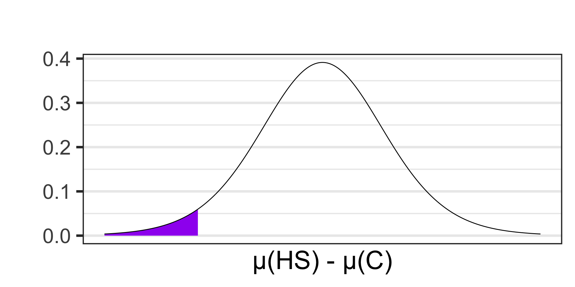
- \(\alpha = 0.10\)
- \(\displaystyle{S_E = 0.3556,~~~\text{df} = \min\left\{n_1 - 1, n_2 - 1\right\}}\)
- \(\displaystyle{t \approx - 1.97}\)
- \(p\)-value \(\approx\) ?
Hypothesis Test for a Difference in Population Means
Scenario: Researchers are interested in understanding how social media usage varies between different educational stages. They surveyed a sample of 14 high school and 21 college students to measure the average time they spend on social media platforms daily. The average time spent for high school students was 2.8 hours per day with a standard deviation of 0.9 hours. For college students, the average was 3.5 hours per day with a standard deviation of 1.2 hours. Conduct a test at the 10% level of significance to determine whether this sample provides evidence to suggest that college students spend more time per day on social media than high school students.
- \(\begin{array}{lcl} H_0 & : & \mu_{\text{HS}} - \mu_{\text{C}} = 0\\ H_a & : & \mu_{\text{HS}} - \mu_{\text{C}} < 0\end{array}\)
- Samples satisfying \(H_a\) are:

- \(\alpha = 0.10\)
- \(\displaystyle{S_E = 0.3556,~~~\text{df} = \min\left\{n_1 - 1, n_2 - 1\right\}}\)
- \(\displaystyle{t \approx - 1.97}\)
- \(p\)-value \(\approx\)
pt(-1.97, df = 13)\(\approx\) 0.0352605
- \(p\)-value \(< \alpha\), reject \(H_0\) and accept \(H_a\)
Hypothesis Test for a Difference in Population Means
Scenario: Researchers are interested in understanding how social media usage varies between different educational stages. They surveyed a sample of 14 high school and 21 college students to measure the average time they spend on social media platforms daily. The average time spent for high school students was 2.8 hours per day with a standard deviation of 0.9 hours. For college students, the average was 3.5 hours per day with a standard deviation of 1.2 hours. Conduct a test at the 10% level of significance to determine whether this sample provides evidence to suggest that college students spend more time per day on social media than high school students.
- Our sample data is not compatible with a reality in which high school students spend the same amount of time per day on social media as college students. College students spend more time.
Confidence Interval for a Population Mean (Together)
Scenario: City planners are investigating the average commute time for residents to work. They survey 17 residents to estimate the average commute time in minutes. The average commute time in the sample was 35 minutes with a standard deviation of 10 minutes. Find a 95% confidence interval for the average commute time.
Confidence Interval for a Difference in Population Means
Scenario: A city council is evaluating the efficiency of two emergency services (ambulance and fire department) based on their average response times. They collect data from 40 recent incidents handled by the ambulance service and 35 recent incidents that the Fire Department responded to. The average response time for the ambulance service was 8 minutes with a standard deviation of 2 minutes, while the average response time for the fire department was 10 minutes with a standard deviation of 2.5 minutes. Build a 98% confidence interval for the difference in average response times.
- Build a confidence interval for the difference in average response times
- \(\displaystyle{\left(\begin{array}{c} \text{Point}\\ \text{Estimate}\end{array}\right) \pm \left(\begin{array}{c} \text{Critical}\\ \text{Value}\end{array}\right)\cdot S_E}\)
- Point estimate for the difference in average response times…
\[\bar{x}_F - \bar{x}_A = 10 - 8 = 2\]
- \(S_E = ?\)
Confidence Interval for a Difference in Population Means
Scenario: A city council is evaluating the efficiency of two emergency services (ambulance and fire department) based on their average response times. They collect data from 40 recent incidents handled by the ambulance service and 35 recent incidents that the Fire Department responded to. The average response time for the ambulance service was 8 minutes with a standard deviation of 2 minutes, while the average response time for the fire department was 10 minutes with a standard deviation of 2.5 minutes. Build a 98% confidence interval for the difference in average response times.
- Build a confidence interval for the difference in average response times
- \(\displaystyle{\left(\begin{array}{c} \text{Point}\\ \text{Estimate}\end{array}\right) \pm \left(\begin{array}{c} \text{Critical}\\ \text{Value}\end{array}\right)\cdot S_E}\)
- Point estimate for the difference in average response times…
\[\bar{x}_F - \bar{x}_A = 10 - 8 = 2\]
- \(\displaystyle{S_E = \sqrt{\frac{s_1^2}{n_1} + \frac{s_2^2}{n_2}},~~~~df = \min\left\{n_1 - 1, n_2 - 1\right\}}\)
Confidence Interval for a Difference in Population Means
Scenario: A city council is evaluating the efficiency of two emergency services (ambulance and fire department) based on their average response times. They collect data from 40 recent incidents handled by the ambulance service and 35 recent incidents that the Fire Department responded to. The average response time for the ambulance service was 8 minutes with a standard deviation of 2 minutes, while the average response time for the fire department was 10 minutes with a standard deviation of 2.5 minutes. Build a 98% confidence interval for the difference in average response times.
- Build a confidence interval for the difference in average response times
- \(\displaystyle{\left(\begin{array}{c} \text{Point}\\ \text{Estimate}\end{array}\right) \pm \left(\begin{array}{c} \text{Critical}\\ \text{Value}\end{array}\right)\cdot S_E}\)
- Point estimate for the difference in average response times…
\[\bar{x}_F - \bar{x}_A = 10 - 8 = 2\]
- \(\displaystyle{S_E = \sqrt{\frac{2^2}{40} + \frac{2.5^2}{35}},~~~~df = \min\left\{n_1 - 1, n_2 - 1\right\}}\)
Confidence Interval for a Difference in Population Means
Scenario: A city council is evaluating the efficiency of two emergency services (ambulance and fire department) based on their average response times. They collect data from 40 recent incidents handled by the ambulance service and 35 recent incidents that the Fire Department responded to. The average response time for the ambulance service was 8 minutes with a standard deviation of 2 minutes, while the average response time for the fire department was 10 minutes with a standard deviation of 2.5 minutes. Build a 98% confidence interval for the difference in average response times.
- Build a confidence interval for the difference in average response times
- \(\displaystyle{\left(\begin{array}{c} \text{Point}\\ \text{Estimate}\end{array}\right) \pm \left(\begin{array}{c} \text{Critical}\\ \text{Value}\end{array}\right)\cdot S_E}\)
- Point estimate for the difference in average response times…
\[\bar{x}_F - \bar{x}_A = 10 - 8 = 2\]
- \(\displaystyle{S_E \approx 0.5278,~~~~df = \min\left\{n_1 - 1, n_2 - 1\right\}}\)
- Critical Value…
Confidence Interval for a Difference in Population Means
Scenario: A city council is evaluating the efficiency of two emergency services (ambulance and fire department) based on their average response times. They collect data from 40 recent incidents handled by the ambulance service and 35 recent incidents that the Fire Department responded to. The average response time for the ambulance service was 8 minutes with a standard deviation of 2 minutes, while the average response time for the fire department was 10 minutes with a standard deviation of 2.5 minutes. Build a 98% confidence interval for the difference in average response times.
- Build a confidence interval for the difference in average response times
- \(\displaystyle{\left(\begin{array}{c} \text{Point}\\ \text{Estimate}\end{array}\right) \pm \left(\begin{array}{c} \text{Critical}\\ \text{Value}\end{array}\right)\cdot S_E}\)
- Point estimate for the difference in average response times…
\[\bar{x}_F - \bar{x}_A = 10 - 8 = 2\]
- \(\displaystyle{S_E \approx 0.5278,~~~~df = \min\left\{n_1 - 1, n_2 - 1\right\}}\)
- Critical Value:
qt(1 - 0.01, df = 34)\(\approx\) 2.44
- \(2 \pm 2.44\cdot\left(0.5278\right)\)
Confidence Interval for a Difference in Population Means
Scenario: A city council is evaluating the efficiency of two emergency services (ambulance and fire department) based on their average response times. They collect data from 40 recent incidents handled by the ambulance service and 35 recent incidents that the Fire Department responded to. The average response time for the ambulance service was 8 minutes with a standard deviation of 2 minutes, while the average response time for the fire department was 10 minutes with a standard deviation of 2.5 minutes. Build a 98% confidence interval for the difference in average response times.
- Build a confidence interval for the difference in average response times
- \(\displaystyle{\left(\begin{array}{c} \text{Point}\\ \text{Estimate}\end{array}\right) \pm \left(\begin{array}{c} \text{Critical}\\ \text{Value}\end{array}\right)\cdot S_E}\)
- Point estimate for the difference in average response times…
\[\bar{x}_F - \bar{x}_A = 10 - 8 = 2\]
- \(\displaystyle{S_E \approx 0.5278,~~~~df = \min\left\{n_1 - 1, n_2 - 1\right\}}\)
- Critical Value:
qt(1 - 0.01, df = 34)\(\approx\) 2.44 - \(2 \pm 2.44\cdot\left(0.5278\right)\)
\[\to \left\{\begin{array}{lcl} 2 - 1.2878 & = & 0.7122\\ 2 + 1.2878 & = & 3.2878\end{array}\right.\]
Confidence Interval for a Difference in Population Means
Scenario: A city council is evaluating the efficiency of two emergency services (ambulance and fire department) based on their average response times. They collect data from 40 recent incidents handled by the ambulance service and 35 recent incidents that the Fire Department responded to. The average response time for the ambulance service was 8 minutes with a standard deviation of 2 minutes, while the average response time for the fire department was 10 minutes with a standard deviation of 2.5 minutes. Build a 98% confidence interval for the difference in average response times.
- We are 98% confident that the difference in average response times in the emergency services is between 0.7122 minutes (about 42.7 seconds) and 3.2878 minutes (about 3 minutes and 17.3 seconds), with the Fire Department taking longer to respond.
Examples to Try
The following slides contain several examples to try
As usual, there are more than we’ll be able to complete during this class meeting
The examples include a mixture of scenarios involving a single population mean or comparison between two population means
The examples also include a mixture of questions which are best answered with confidence intervals or best answered with hypothesis tests
You’ll need to determine which scenario you are in and which tools to apply
Examples to Try: Daily Coffee Consumption
Scenario: A coffee company is interested in the average amount of coffee consumed by office workers per day. They survey a sample of 22 office workers to estimate this average and observe a mean consumption of 3.2 cups with a standard deviation of 1.1 cups. Construct a 90% confidence interval for the average number of cups of coffee consumed per day by office workers.
Examples to Try: Average Sleep Time
Scenario: A university researcher investigates whether students in a demanding academic program sleep less on average than those in a less rigorous program. They survey two samples of students, including 45 from a very rigorous program and 50 from a less rigorous program. The average sleep time for students in the very rigorous program was 6.2 hours with a standard deviation of 1.3 hours. The students in the less rigorous program averaged 7.5 hours of sleep with a standard deviation of 1 hour. Construct a 95% confidence interval for the difference in average sleep.
Examples to Try: Bird Migration
Scenario: Ornithologists studying a specific species of migratory bird believe the average duration of one leg of their migration flight is about 6 hours. They observe a sample of 25 birds this season and find a mean flight duration of 5.5 hours with a standard deviation of 1.2 hours. Does this sample provide evidence to suggest that the duration differs from 6 hours?
Examples to Try: Daily Step Counts
Scenario: A company has introduced a new wellness program aimed at increasing employees’ daily step count. Prior to the program, the average daily step count was 6,000 steps. After one month, a sample of 50 employees reports a mean step count of 6,400 steps with a standard deviation of 1,200 steps. Find a 90% confidence interval for the average daily step count after implementing this new wellness program.
Examples to Try: Water Consumption
Scenario: Public health officials are examining differences in hydration habits between two cities. They survey 50 residents from each city to determine how much water they consume on average each day to promote health awareness initiatives. The mean water consumption in City A was 2.7 liters, with a standard deviation of 1.2 liters. The average water consumption in City B was 3.1 liters, with a standard deviation of 1.4 liters. Conduct a test to determine whether the sample provides evidence for a difference in average water consumption between the two cities.
Examples to Try: Starting Salaries
Scenario: A career services office at a university wants to estimate the average starting salary of its recent graduates. They collect data from a sample of 34 graduates who landed jobs after graduation and found an average salary of $52,000 with a standard deviation of $8,000. Construct a 95% confidence interval for the average starting salary of recent graduates.
Exit Ticket Task
Navigate to our MAT241 Exit Ticket Form, answer the questions, and complete the task below.
Note. Today’s discussion is listed as 14. Inference for Means

Task: A hospital is evaluating whether a new early-discharge protocol has reduced the average length of stay for patients admitted with uncomplicated pneumonia. Historically, the average length of stay for these patients was 4.8 days. After implementing the new protocol, a random sample of 36 patients had an average length of stay of 4.3 days with a standard deviation of 1.2 days. Describe the steps required to construct a confidence interval for the average length of stay under this new protocol.
Next Time…
Lots of Practice