Introduction to Inference: The Central Limit Theorem

The Highlights

Reminder on probability with the normal distribution
Review of means versus proportions
Sampling from a population (working with a Population Distribution)
Drawing Multiple Observations (Collecting a Sample)
- Question: Can we calculate probabilities associated with sample outcomes in a familiar manner?
What is the Sampling Distribution?
- A few examples with means and proportions
- When is a sampling distribution [nearly] normal?
Central Limit Theorem
- CLT for means and CLT for proportions
- Examples: Probabilities associated with random samples summarized by means or proportions
Summary

Probability and the Normal Distribution (A Reminder)

A normal distribution is defined by its mean ($\mu$) and standard deviation ($\sigma$)

The mean, $\mu$, is the center of the distribution
The standard deviation, $\sigma$, governs the spread of the distribution – a larger $\sigma$ means a wider distribution, while a smaller $\sigma$ means a more narrow distribution

Probabilities associated with values far away from the mean are larger in the distribution on the left than they are in the distribution on the right.

Probability and the Normal Distribution (A Reminder)

Probabilities associated with values far away from the mean are larger in the distribution on the left than they are in the distribution on the right.

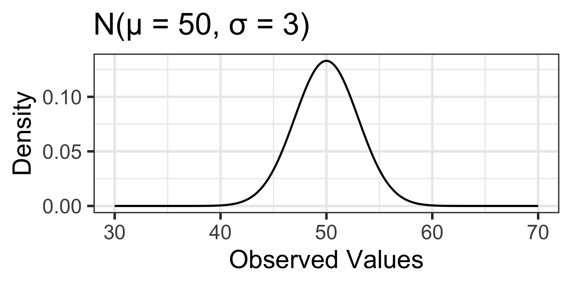
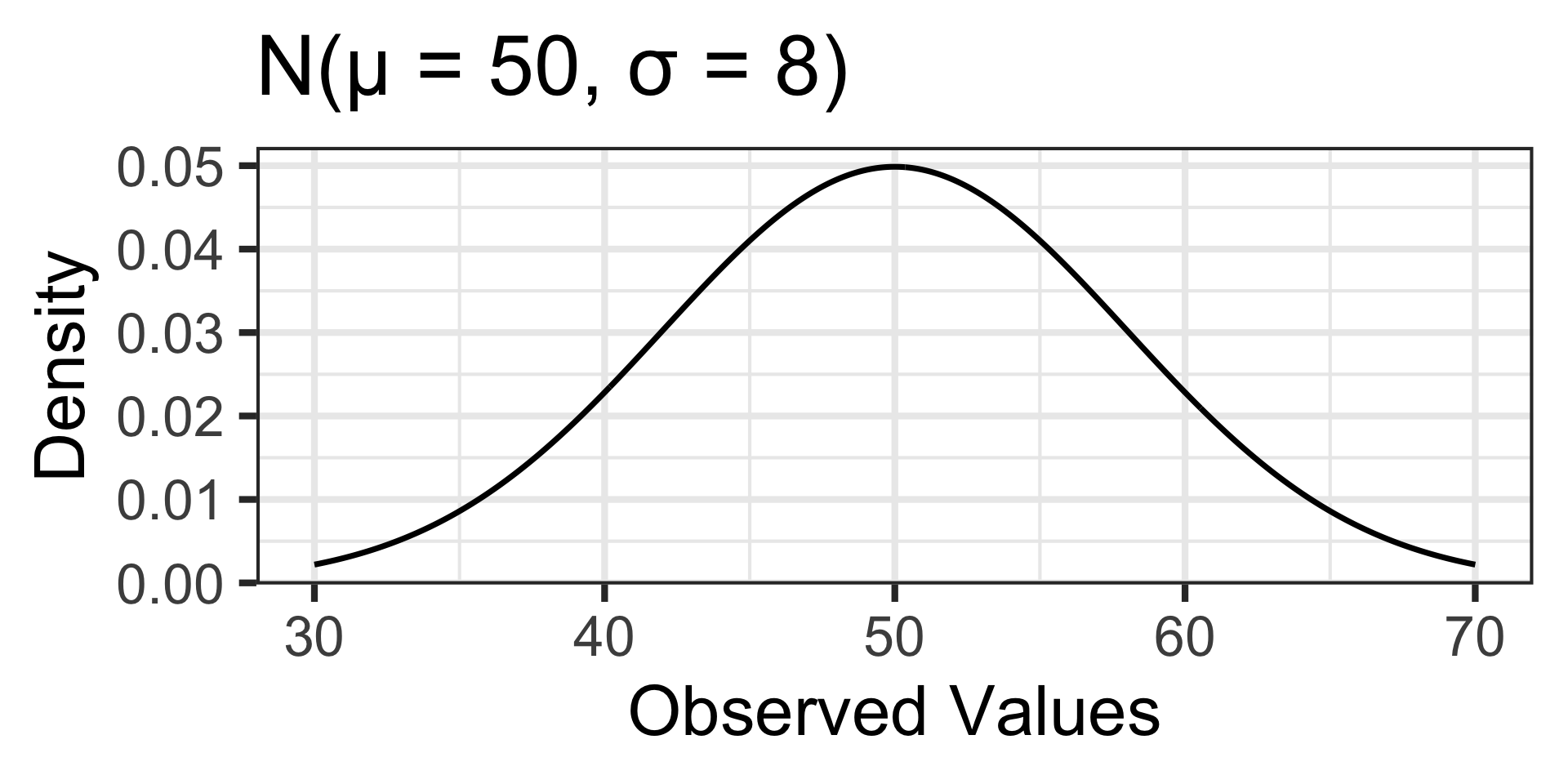
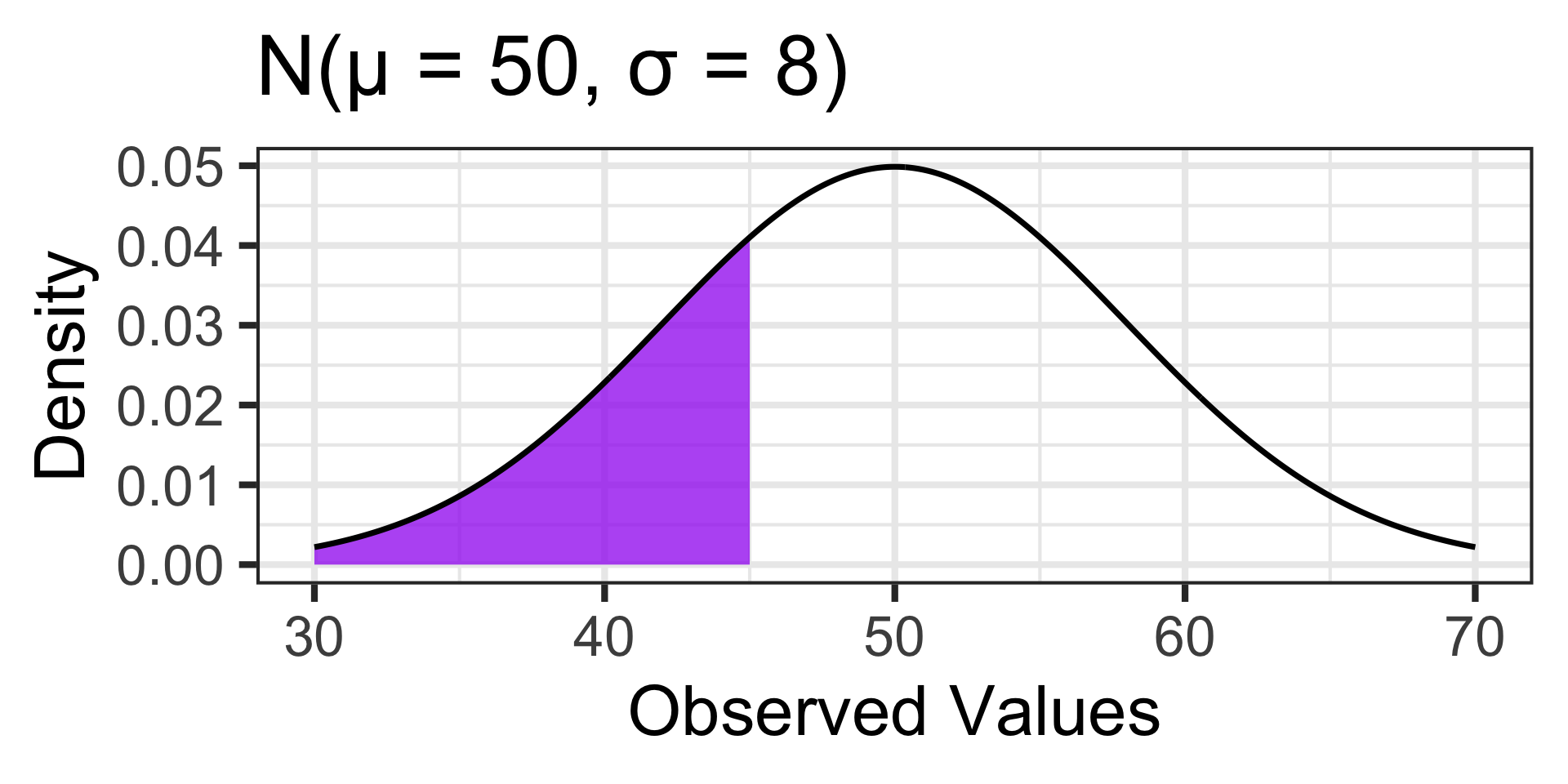
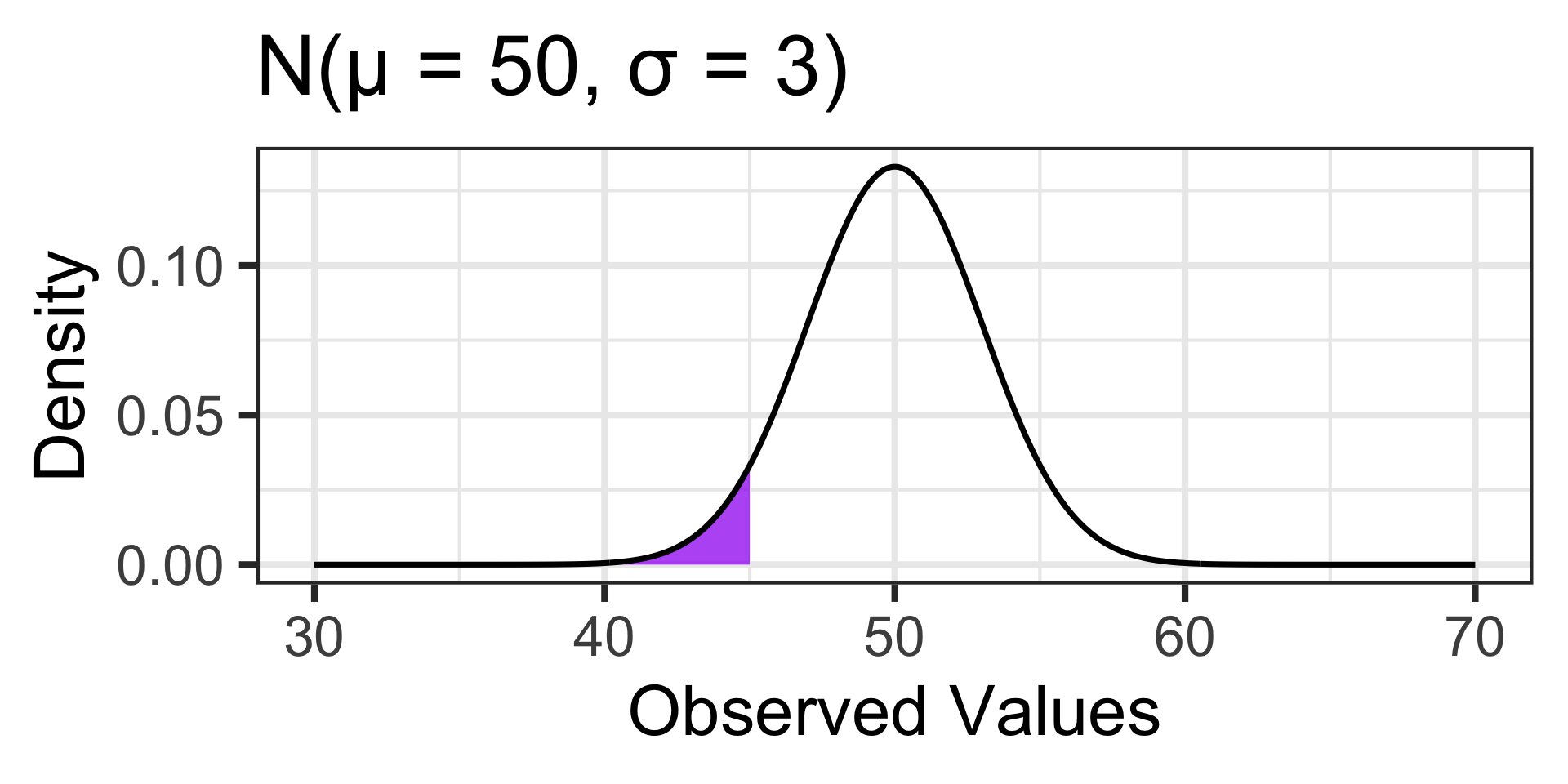
$\mathbb{P}\left[X < 45\right] \approx ...$

Probability and the Normal Distribution (A Reminder)

Probabilities associated with values far away from the mean are larger in the distribution on the left than they are in the distribution on the right.

$\mathbb{P}\left[X < 45\right] \approx ...$

pnorm(45, 50, 8) $\approx$ 0.266

pnorm(45, 50, 3) $\approx$ 0.0478

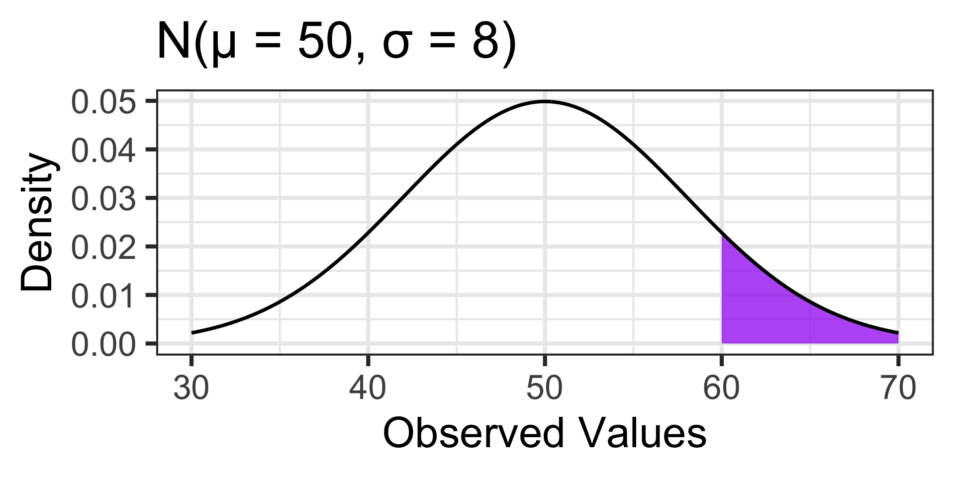
Probability and the Normal Distribution (A Reminder)

Probabilities associated with values far away from the mean are larger in the distribution on the left than they are in the distribution on the right.

$\mathbb{P}\left[X \geq 60\right] \approx ...$

Probability and the Normal Distribution (A Reminder)

Probabilities associated with values far away from the mean are larger in the distribution on the left than they are in the distribution on the right.

$\mathbb{P}\left[X \geq 60\right] \approx ...$

1 - pnorm(60, 50, 8) $\approx$ 0.1056

1 - pnorm(60, 50, 3) $\approx$ 0.0004

Means versus Proportions (Review)

We use means to summarize numerical data

Result from questions that have numerical responses like
- “How many hours a day are you focused on looking at a screen?”
- “What is the white blood cell count in this blood sample?”
- “How many rushing yards did the running back gain?”

We use proportions to summarize categorical data

Result from questions questions that have a categorical response like
- “Do you intend to vote in the next presidential election?”
- “Is the result of the game a win, loss, or draw?”
- “Is the median family income in this neighborhood at or below $30,000, between $30,001 and $58,020, between $58,021 and $94,000, between $94,001 and $153,000, or greater than $153,000?” ¹

A Note on Proportions and the Binomial Distribution

We use proportions to summarize categorical data

Result from questions questions that have a categorical response like
- “Do you intend to vote in the next presidential election?”
- “Is the result of the game a win, loss, or draw?”
- “Is the median family income in this neighborhood at or below $30,000, between $30,001 and $58,020, between $58,021 and $94,000, between $94,001 and $153,000, or greater than $153,000?” ¹

Note: All of the above questions can be analysed with a binomial distribution as long as we classify one level (category) as a success and group the others together as failure.

Sampling One Observation at a Time (Population Distribution)

The distances traveled by a 10lb pumpkin launched via a trebuchet are approximately normally distributed with a mean of 1800ft and a standard deviation of 250ft. Find the probability that a launched pumpkin exceeds 2000ft.

Sampling One Observation at a Time (Population Distribution)

The distances traveled by a 10lb pumpkin launched via a trebuchet are approximately normally distributed with a mean of 1800ft and a standard deviation of 250ft. Find the probability that a launched pumpkin exceeds 2000ft.

$\mathbb{P}\left[X > 2000\right] \approx ...$

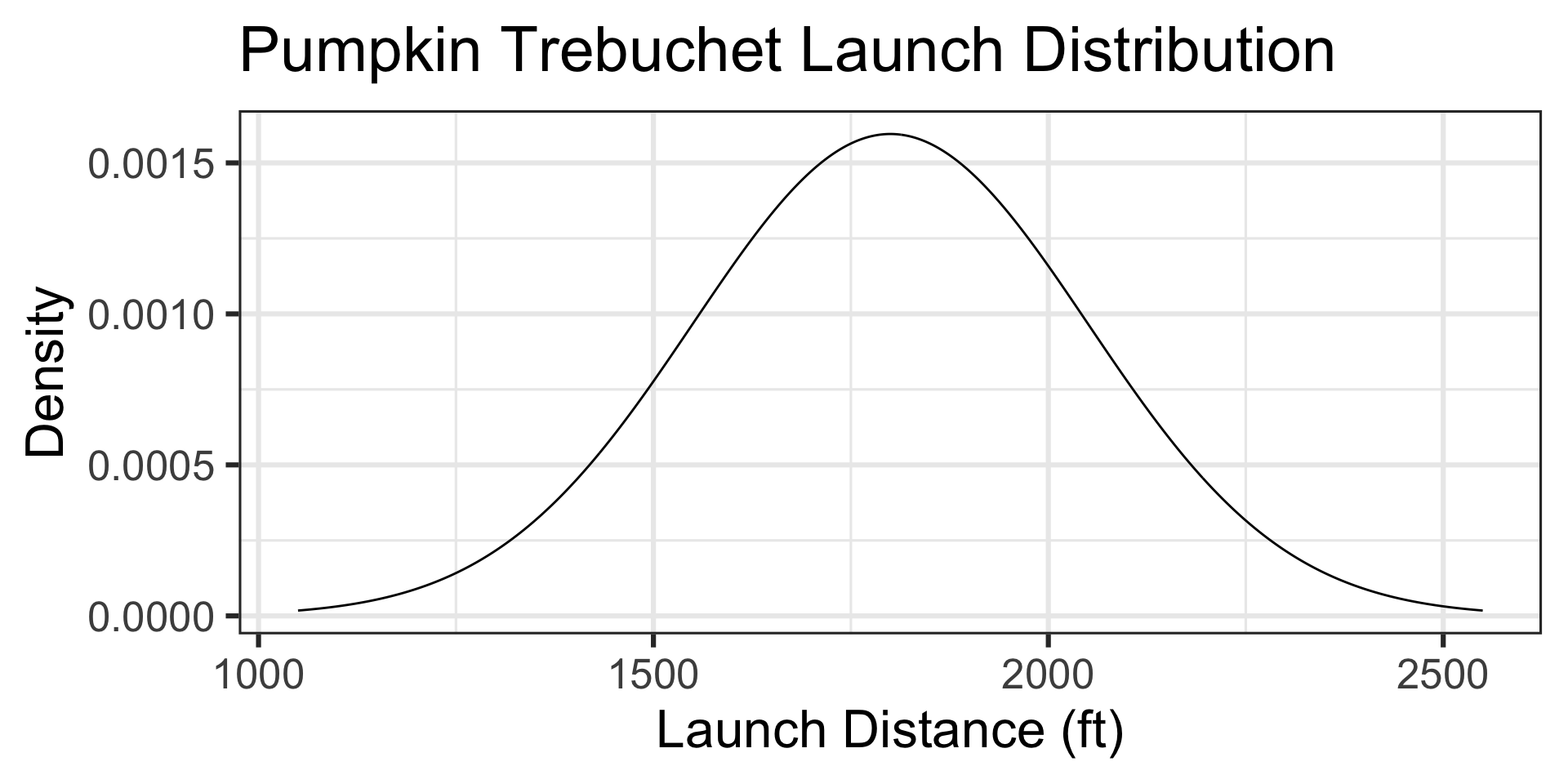
Sampling One Observation at a Time (Population Distribution)

The distances traveled by a 10lb pumpkin launched via a trebuchet are approximately normally distributed with a mean of 1800ft and a standard deviation of 250ft. Find the probability that a launched pumpkin exceeds 2000ft.

$\mathbb{P}\left[X > 2000\right] \approx ...$

1 - pnorm(2000, mean = 1800, sd = 250) $\approx$ 0.2118554

Sampling One Observation at a Time (Population Distribution)

The distances traveled by a 10lb pumpkin launched via a trebuchet are approximately normally distributed with a mean of 1800ft and a standard deviation of 250ft. Find the probability that a launched pumpkin exceeds 2000ft.

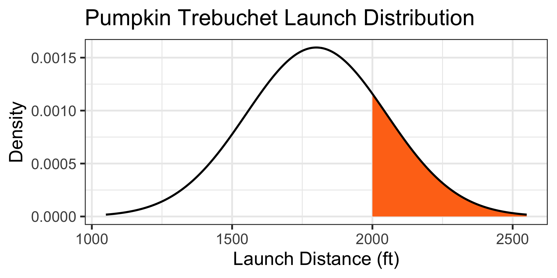
$\mathbb{P}\left[X > 2000\right] \approx ...$

1 - pnorm(2000, mean = 1800, sd = 250) $\approx$ 0.2118554

There’s about a 21.19% chance that a randomly selected pumpkin will be launched further than 2,000ft.

Motivating Example: A Confident Team…

Motivating Example: A particular team feels that their pumpkin launching trebuchet is much better than average. On a typical day (it’s not extra windy), the team launches a random selection of twelve 10lb pumpkins. Their average launch distance is 2,028ft. What is the probability that a random selection of twelve launches averages 2,028ft or further?

Question 1: Should it be the same as the probability that a single launch exceeds 2,028ft?

Question 2: What needs to happen for a collection of launches to average 2,028ft?

What if one of the twelve launches was a relatively short, but not unexpected, launch of say 1700ft?

Motivating Example: A Confident Team…

Motivating Example: A particular team feels that their pumpkin launching trebuchet is much better than average. On a typical day (it’s not extra windy), the team launches a random selection of twelve 10lb pumpkins. Their average launch distance is 2,028ft. What is the probability that a random selection of twelve launches averages 2,028ft or further?

A Simulation: Let’s simulate the launches of 12 randomly selected 10lb pumpkins…

Motivating Example: A Confident Team…

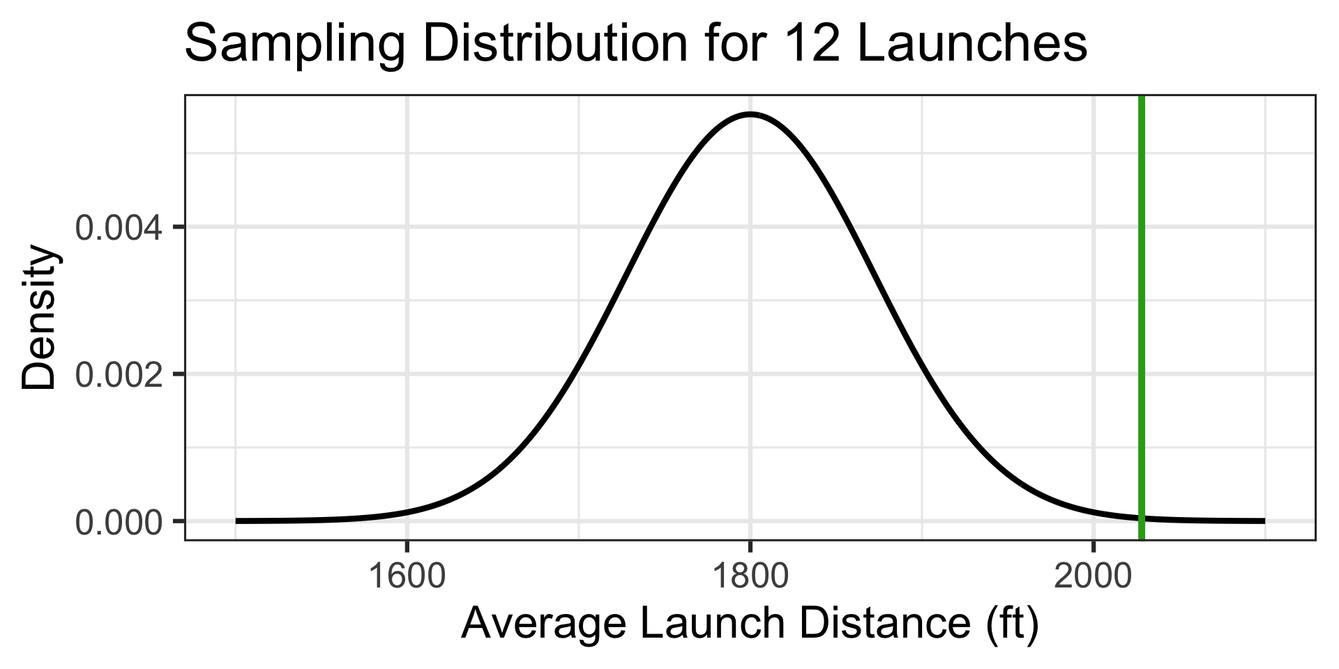
Motivating Example: A particular team feels that their pumpkin launching trebuchet is much better than average. On a typical day (it’s not extra windy), the team launches a random selection of twelve 10lb pumpkins. Their average launch distance is 2,028ft. What is the probability that a random selection of twelve launches averages 2,028ft or further?

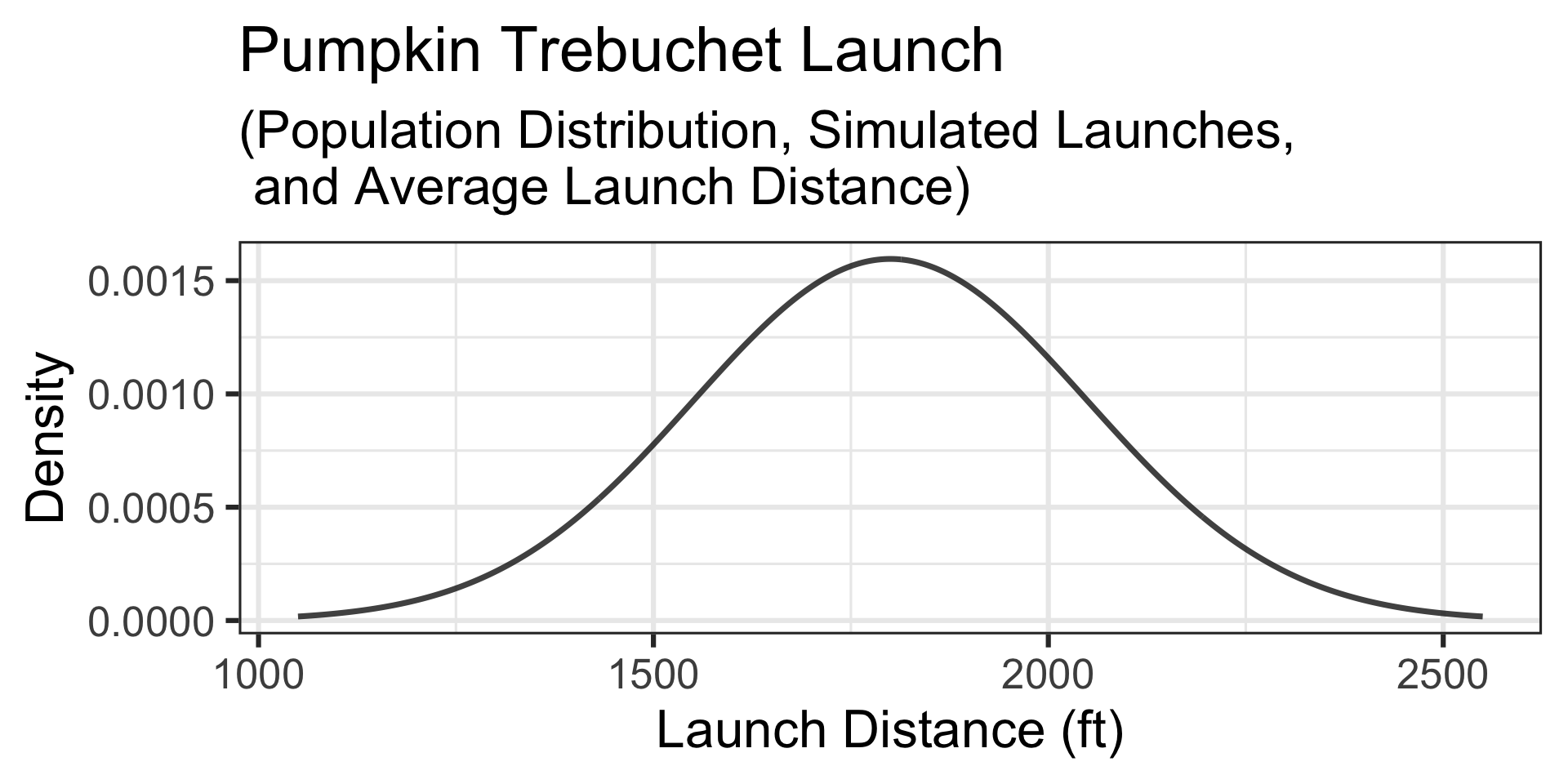
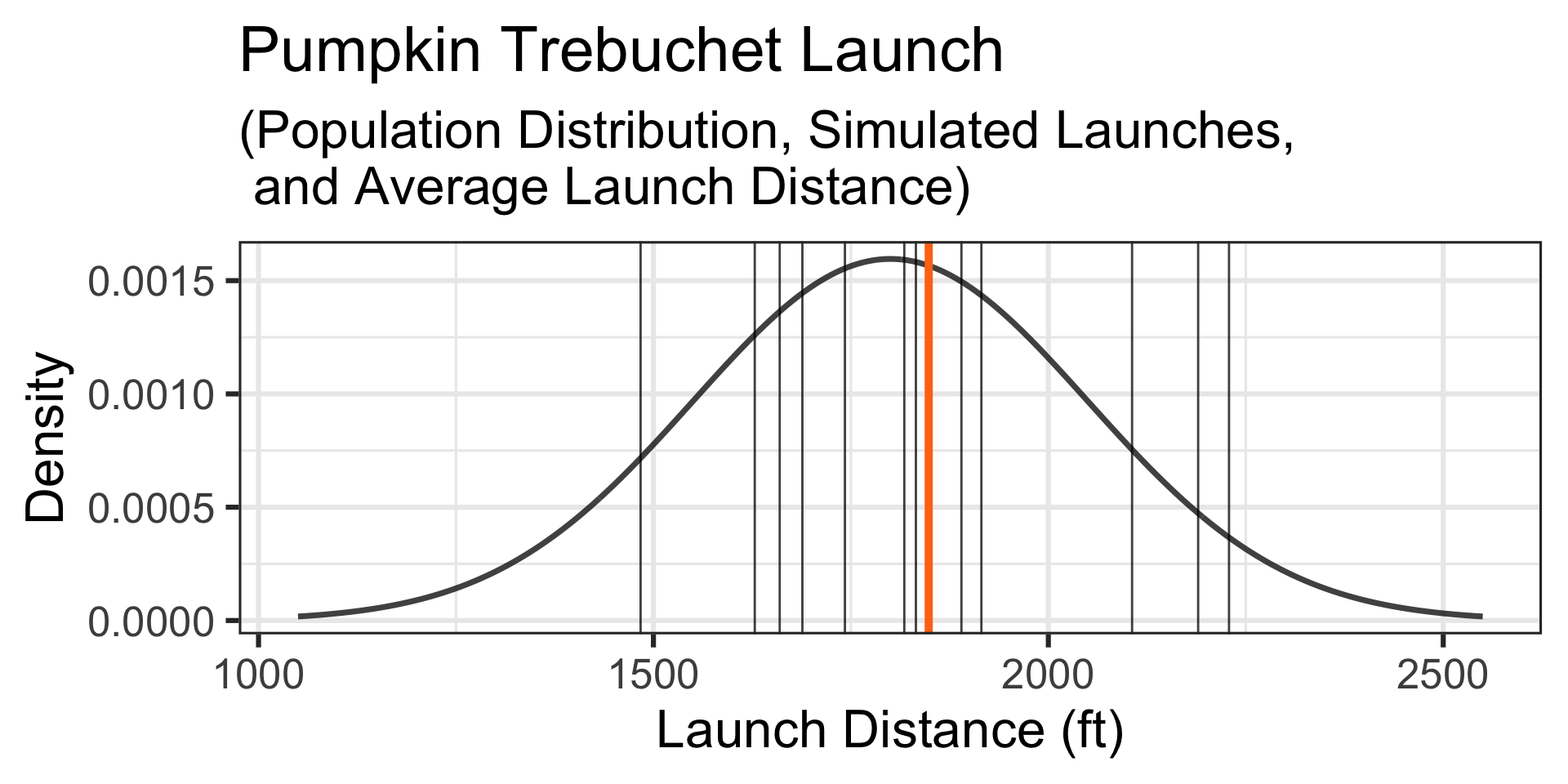
A Simulation: Let’s simulate the launches of 12 randomly selected 10lb pumpkins…

Motivating Example: A Confident Team…

Motivating Example: A particular team feels that their pumpkin launching trebuchet is much better than average. On a typical day (it’s not extra windy), the team launches a random selection of twelve 10lb pumpkins. Their average launch distance is 2,028ft. What is the probability that a random selection of twelve launches averages 2,028ft or further?

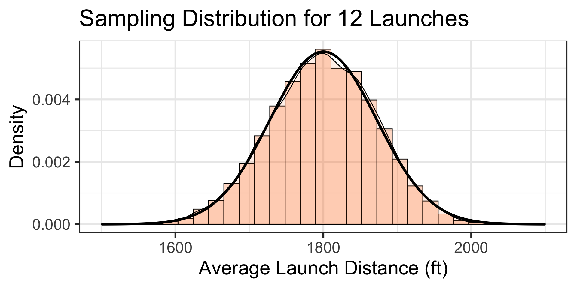
A Simulation: Let’s simulate the launches of 12 randomly selected 10lb pumpkins… The simulated launch distances appear below and the launches, along their average launch distance are shown by the vertical lines on the graph to the right.

Motivating Example: A Confident Team…

Motivating Example: A particular team feels that their pumpkin launching trebuchet is much better than average. On a typical day (it’s not extra windy), the team launches a random selection of twelve 10lb pumpkins. Their average launch distance is 2,028ft. What is the probability that a random selection of twelve launches averages 2,028ft or further?

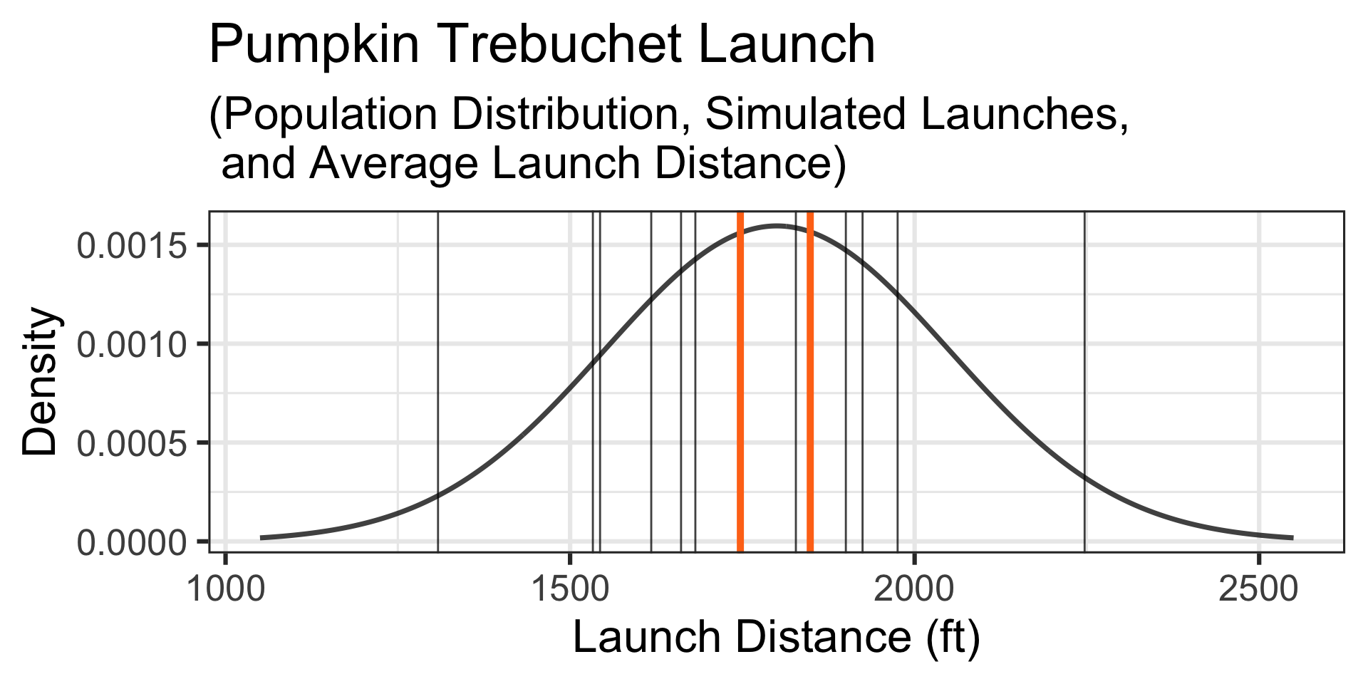
A Simulation: Let’s simulate another set of launches of 12 randomly selected 10lb pumpkins… The simulated launch distances appear below and the launches, along their average launch distance and the average launch distance from our first set of launches are shown on the graph to the right.

Motivating Example: A Confident Team…

Motivating Example: A particular team feels that their pumpkin launching trebuchet is much better than average. On a typical day (it’s not extra windy), the team launches a random selection of twelve 10lb pumpkins. Their average launch distance is 2,028ft. What is the probability that a random selection of twelve launches averages 2,028ft or further?

A Simulation: Let’s simulate another set of launches of 12 randomly selected 10lb pumpkins… The simulated launch distances appear below and the launches, along their average launch distance and the average launch distance from our first set of launches are shown on the graph to the right.

Motivating Example: A Confident Team…

Motivating Example: A particular team feels that their pumpkin launching trebuchet is much better than average. On a typical day (it’s not extra windy), the team launches a random selection of twelve 10lb pumpkins. Their average launch distance is 2,028ft. What is the probability that a random selection of twelve launches averages 2,028ft or further?

A Simulation: Okay – we see how this is working, but it’s going slowly. Let’s simulate 50,000 collections of launches of 12 randomly selected 10lb pumpkins.

Motivating Example: A Confident Team…

Motivating Example: A particular team feels that their pumpkin launching trebuchet is much better than average. On a typical day (it’s not extra windy), the team launches a random selection of twelve 10lb pumpkins. Their average launch distance is 2,028ft. What is the probability that a random selection of twelve launches averages 2,028ft or further?

A Simulation: Okay – we see how this is working, but it’s going slowly. Let’s simulate 50,000 collections of launches of 12 randomly selected 10lb pumpkins.

Motivating Example: A Confident Team…

Motivating Example: A particular team feels that their pumpkin launching trebuchet is much better than average. On a typical day (it’s not extra windy), the team launches a random selection of twelve 10lb pumpkins. Their average launch distance is 2,028ft. What is the probability that a random selection of twelve launches averages 2,028ft or further?

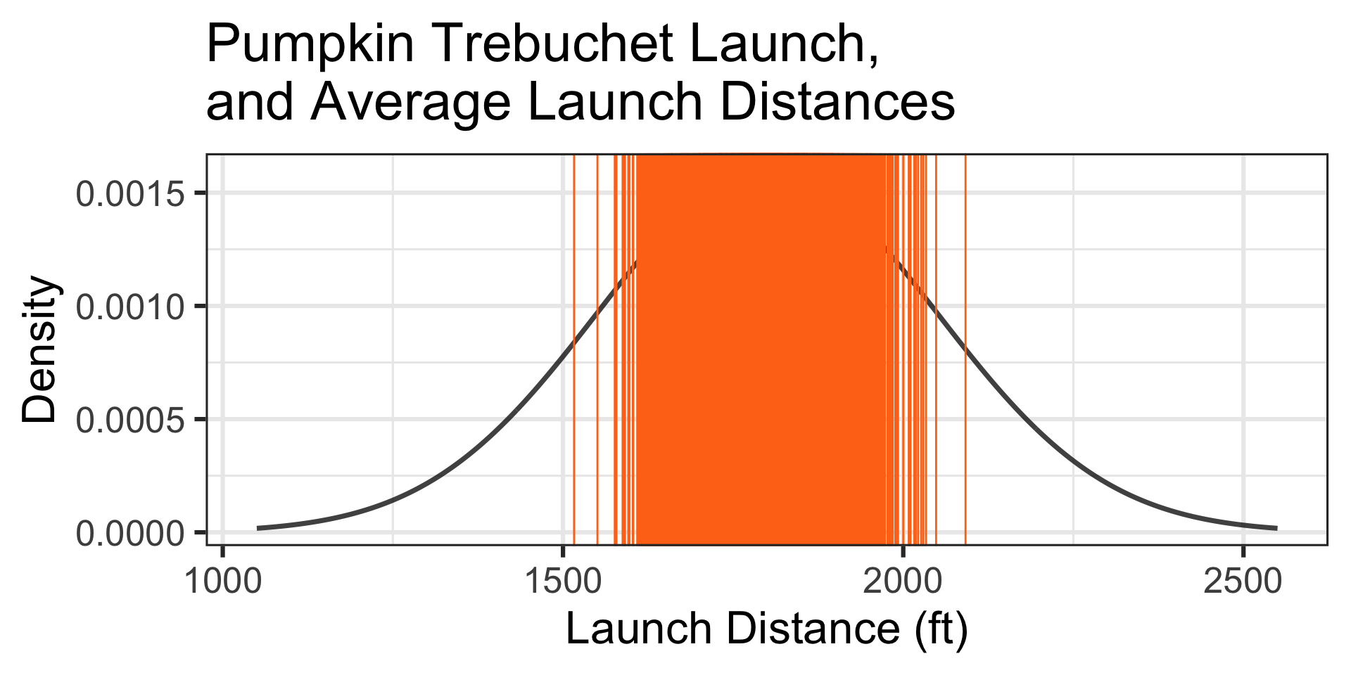
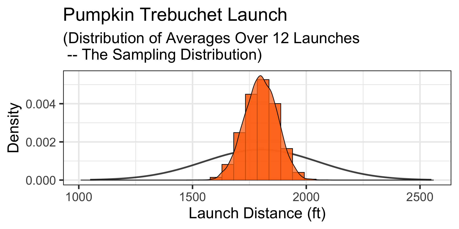
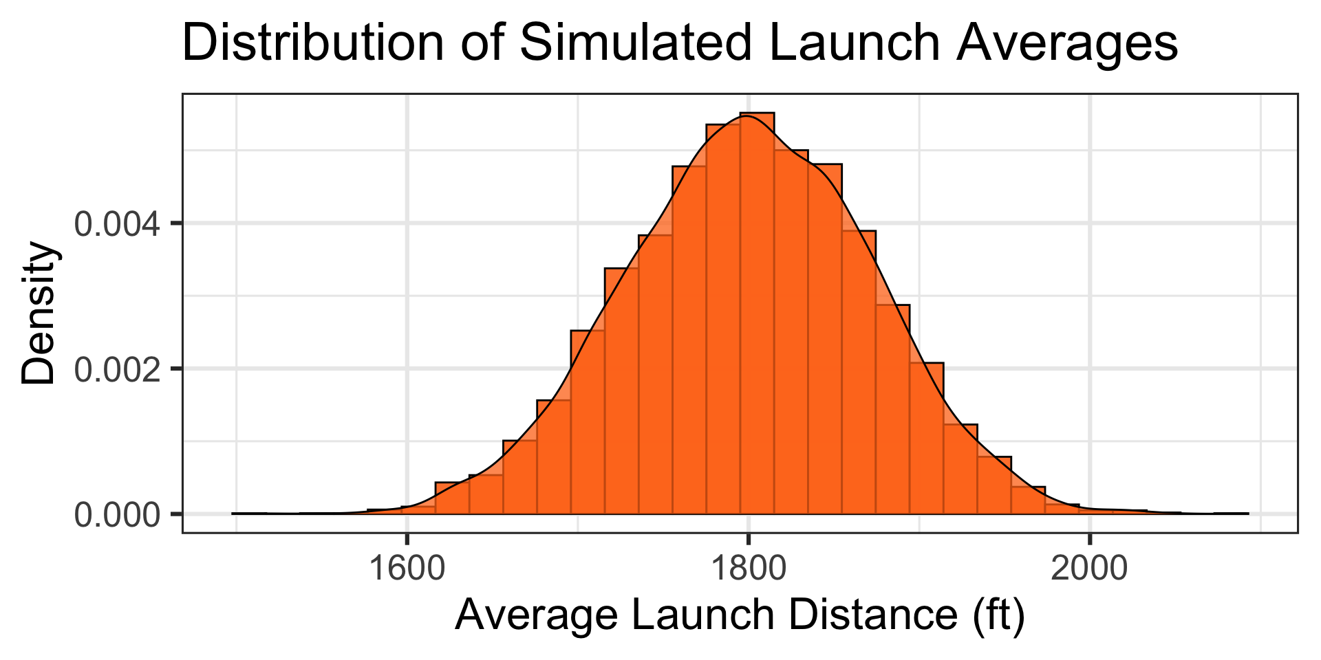
A Simulation: Okay – we see how this is working, but it’s going slowly. Let’s simulate 50,000 collections of launches of 12 randomly selected 10lb pumpkins.

Motivating Example: A Confident Team…

Motivating Example: A particular team feels that their pumpkin launching trebuchet is much better than average. On a typical day (it’s not extra windy), the team launches a random selection of twelve 10lb pumpkins. Their average launch distance is 2,028ft. What is the probability that a random selection of twelve launches averages 2,028ft or further?

A Simulation: Okay – we see how this is working, but it’s going slowly. Let’s simulate 50,000 collections of launches of 12 randomly selected 10lb pumpkins.

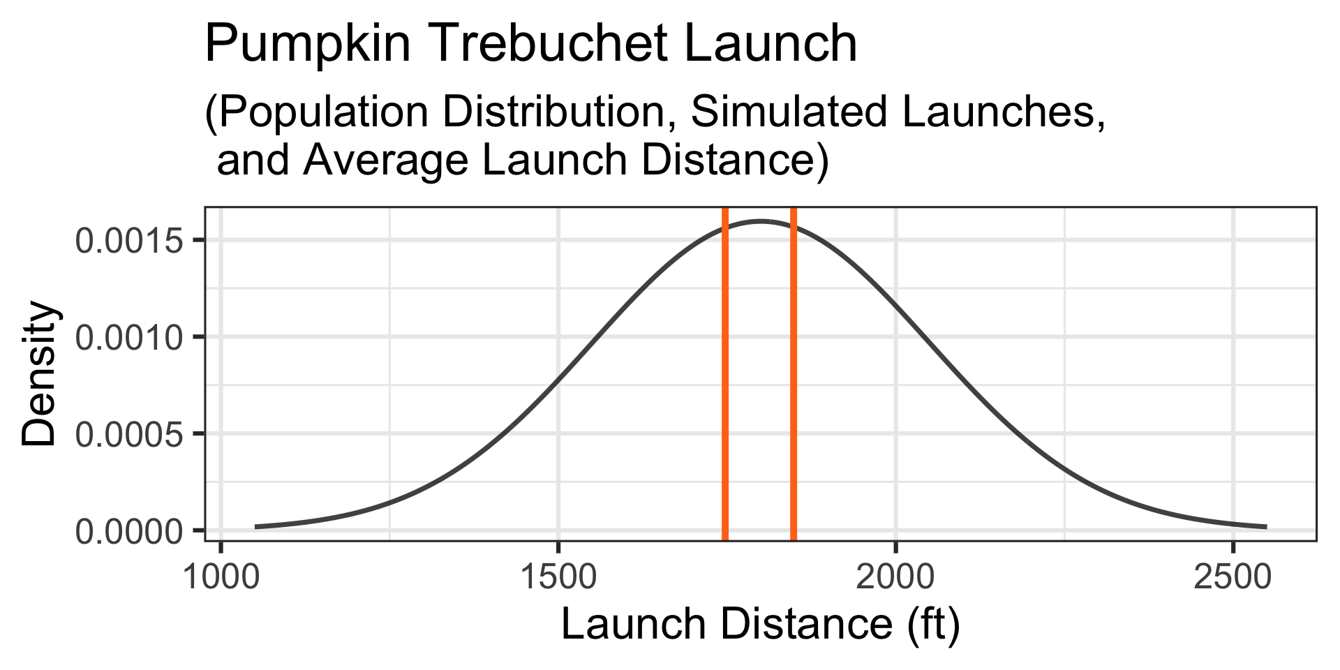
An average launch distance of 2,028ft is at the green vertical line.

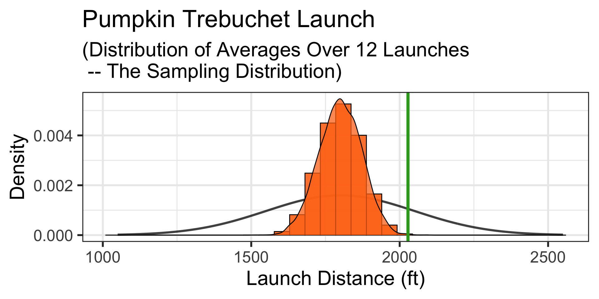
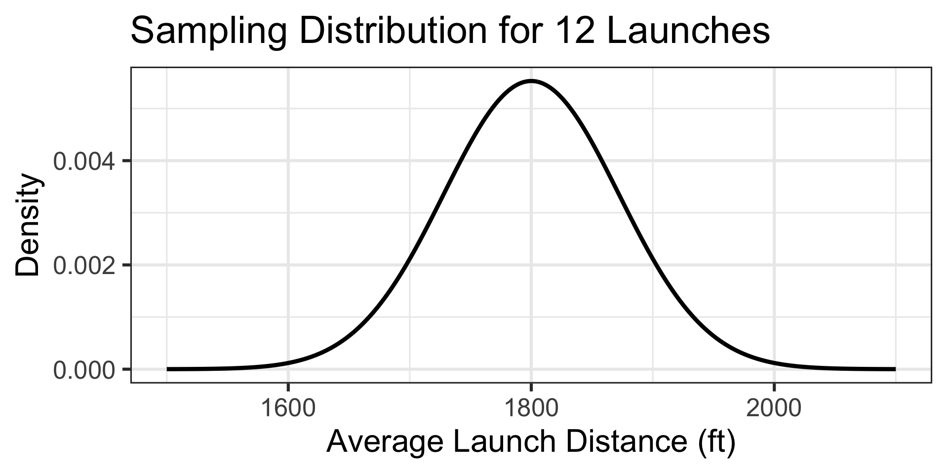
Takeaway: The distribution of averages of 12 launches is much more narrow than the population distribution. The probability of averaging a distance of at least 2,028ft is much lower than the probability of a single launch being at least 2,028ft.

We’ll come back and finish this problem soon, but first we need a detour to talk about this new, more narrow distribution.

What is the Sampling Distribution?

The sampling distribution is a theoretical distribution of summary statistics resulting from samples of the same size. For example,

the distribution of all average launch distances from twelve launches of 10lb pumpkins from a trebuchet.
the distribution of all sample proportions from collections of 100 likely voters asked whether they favor increasing the state’s mandatory judicial retirement age from 70 to 75.

Let’s take a look at some hypothetical population and corresponding sampling distributions.

Hypothetical Population and Sampling Distributions for Means

Flimps, flomps, and flumps are [fictitious] numerical variables whose population distributions appear below and with corresponding sampling distributions to the right.

Sampling distributions are shown for samples of three observations (s3_*), fifteen observations (s15_*), and thirty observations (s30_*).

Hypothetical Population and Sampling Distributions for Proportions

Similarly, grimps, gromps, and grumps are [fictitious] categorical variables for which we can define success and failure. The sampling distributions for proportion corresponding to a successful outcome appears below.

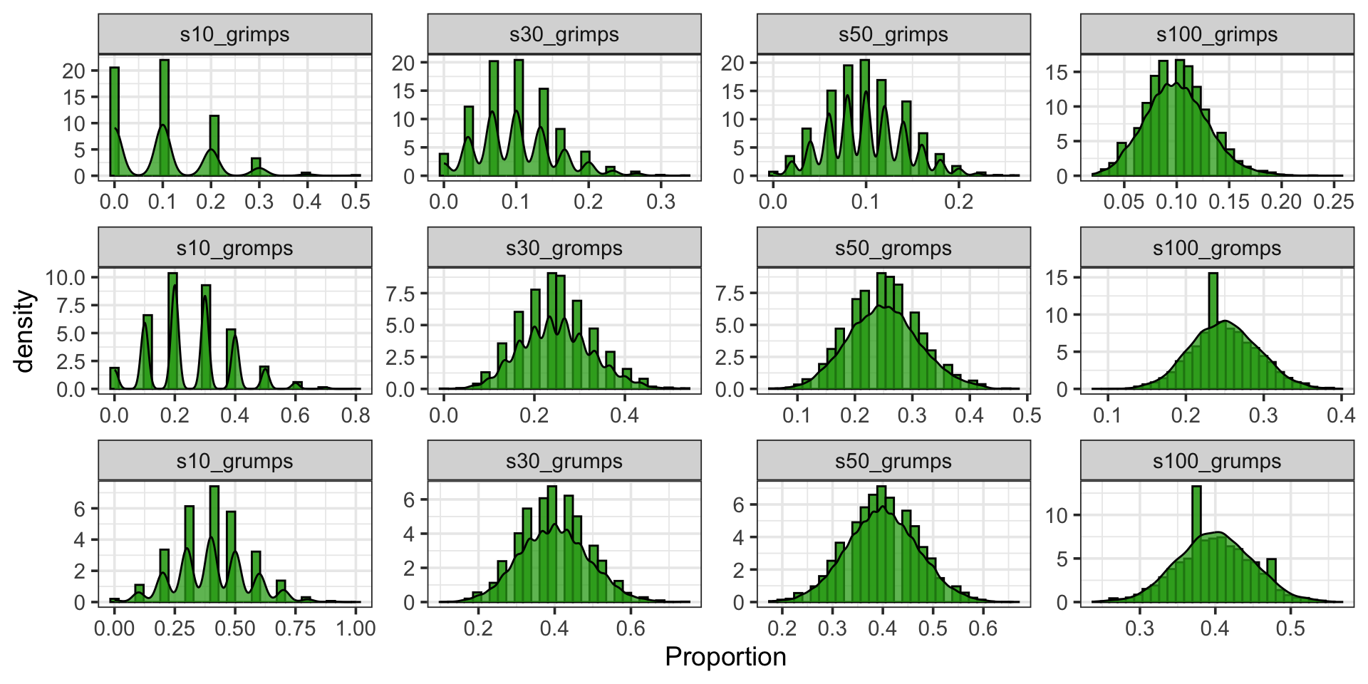
Sampling distributions this time are shown for samples of ten observations (s10_*), thirty observations (s30_*), fifty observations (s50_*), and one hundred observations (s100_*).

When is a Sampling Distribution [Nearly] Normal?

Important: Bringing back our sampling distributions for flimps, flomps, and flumps (numerical variables) we see that the more skewed the population distribution, the larger the sample size required before the sampling distribution is well-approximated by a normal distribution.

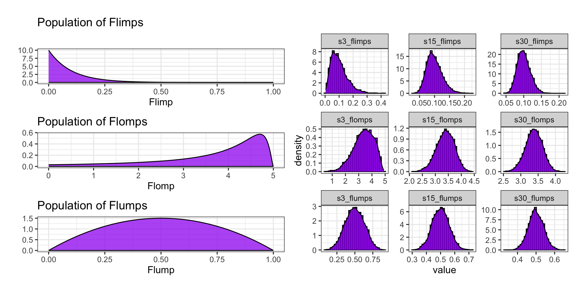
Some people/books recommend $n\geq 30$, but I advocate against this rule of thumb because of the slightly maintained skew we see in the top two rows of plots.

When is a Sampling Distribution [Nearly] Normal?

Important: Bringing back our sampling distributions for grimps, gromps, and grumps (binary categorical variables) we see that the presence of skew is related to the population proportion and the sample size.

As a rule of thumb, the sampling distribution for the population proportion is nearly normal as long as $n\cdot p\geq 10$ and $n\cdot\left(1 - p\right) \geq 10$. That is, we expect at least 10 successes and at least 10 failures.

This is sometimes called the success-failure condition.

The Good News…

We can use the normal distribution as a model for the Sampling Distribution as long as our sample sizes are large enough to overcome any skew in the population distribution (for numerical variables), or large enough that the success-failure condition is satisfied (for binary categorical variables).

The Punchline: We can use our familiar pnorm() and qnorm() functionality when working with Sampling Distributions$^*$

The Central Limit Theorem

Central Limit Theorem (CLT): The Sampling Distribution of the mean (average of averages or average of proportions) is approximately normally distributed as long as the sample sizes are large enough.

The mean of the sampling distribution is…

equal to the population mean ($\mu$) for numerical variables
equal to the population proportion ($p$) for binary categorical variables

The standard deviation of the sampling distribution is called the standard error and is denoted by $S_E$…

The standard error for the sampling distribution of means is $\boxed{~\displaystyle{S_E = \sigma / \sqrt{n}}~}$, where $\sigma$ is the population standard deviation and $n$ is the sample size.
The standard error for the sampling distribution of proportions is $\boxed{~\displaystyle{S_E = \sqrt{\frac{p\left(1 - p\right)}{n}}}~}$ where $p$ is the population proportion (or an estimate for it) and $n$ is the sample size.

The Central Limit Theorem (Restated)

CLT for Means: For large enough sample sizes ($n$), the sampling distribution of the mean is well-approximated by $\displaystyle{N\left(\mu,~S_E = \sigma /\sqrt{n}\right)}$

Note. Recall that $\displaystyle{N\left(\mu,~S_E = \sigma /\sqrt{n}\right)}$ means the “normal distribution centered at $\mu$ and with spread (standard deviation/standared error) described by $\displaystyle{\sigma/\sqrt{n}}$”

CLT for Proportions: For large enough sample sizes ($n$), the sampling distribution of the proportion is well-approximated by $\displaystyle{N\left(p,~S_E = \sqrt{\frac{p\left(1 - p\right)}{n}}\right)}$

Note. Similarly, $\displaystyle{N\left(p,~S_E = \sqrt{\frac{p\left(1 - p\right)}{n}}\right)}$ means the “normal distribution centered at $p$ and with spread (standard deviation/standared error) described by $\displaystyle{\sqrt{\frac{p\left(1 - p\right)}{n}}}$”

Back to Pumpkin Launching!

Reminder: The distances traveled by a 10lb pumpkin launched via a trebuchet are approximately normally distributed with a mean of 1800ft and a standard deviation of 250ft. A particular team feels that their pumpkin launching trebuchet is much better than average. On a typical day (it’s not extra windy), the team launches a random selection of twelve 10lb pumpkins. Their average launch distance is 2,028ft. What is the probability that a random selection of twelve launches averages 2,028ft or further?

Note that the population distribution of launch distances is not skewed (it is approximately normal).
This means that we have no skew to overcome, and our sampling distribution will be approximately normal.
Launch distance is a numerical variable, and so the sampling distribution for average launch distances of 12 pumpkins will be $\displaystyle{N\left(\mu, S_E = \sigma/\sqrt{n}\right)}$, which in this case is $\displaystyle{N\left(\mu = 1800, S_E = 250/\sqrt{12}\right)}$

Back to Pumpkin Launching!

Reminder: The distances traveled by a 10lb pumpkin launched via a trebuchet are approximately normally distributed with a mean of 1800ft and a standard deviation of 250ft. A particular team feels that their pumpkin launching trebuchet is much better than average. On a typical day (it’s not extra windy), the team launches a random selection of twelve 10lb pumpkins. Their average launch distance is 2,028ft. What is the probability that a random selection of twelve launches averages 2,028ft or further?

Note that the population distribution of launch distances is not skewed (it is approximately normal).
This means that we have no skew to overcome, and our sampling distribution will be approximately normal.
Launch distance is a numerical variable, and so the sampling distribution for average launch distances of 12 pumpkins will be $\displaystyle{N\left(\mu, S_E = \sigma/\sqrt{n}\right)}$, which in this case is $\displaystyle{N\left(\mu = 1800, S_E = 250/\sqrt{12}\right)}$

Back to Pumpkin Launching!

Reminder: The distances traveled by a 10lb pumpkin launched via a trebuchet are approximately normally distributed with a mean of 1800ft and a standard deviation of 250ft. A particular team feels that their pumpkin launching trebuchet is much better than average. On a typical day (it’s not extra windy), the team launches a random selection of twelve 10lb pumpkins. Their average launch distance is 2,028ft. What is the probability that a random selection of twelve launches averages 2,028ft or further?

Note that the population distribution of launch distances is not skewed (it is approximately normal).
This means that we have no skew to overcome, and our sampling distribution will be approximately normal.
Launch distance is a numerical variable, and so the sampling distribution for average launch distances of 12 pumpkins will be $\displaystyle{N\left(\mu, S_E = \sigma/\sqrt{n}\right)}$, which in this case is $\displaystyle{N\left(\mu = 1800, S_E = 250/\sqrt{12}\right)}$

Back to Pumpkin Launching!

Reminder: The distances traveled by a 10lb pumpkin launched via a trebuchet are approximately normally distributed with a mean of 1800ft and a standard deviation of 250ft. A particular team feels that their pumpkin launching trebuchet is much better than average. On a typical day (it’s not extra windy), the team launches a random selection of twelve 10lb pumpkins. Their average launch distance is 2,028ft. What is the probability that a random selection of twelve launches averages 2,028ft or further?

Note that the population distribution of launch distances is not skewed (it is approximately normal).
This means that we have no skew to overcome, and our sampling distribution will be approximately normal.
Launch distance is a numerical variable, and so the sampling distribution for average launch distances of 12 pumpkins will be $\displaystyle{N\left(\mu, S_E = \sigma/\sqrt{n}\right)}$, which in this case is $\displaystyle{N\left(\mu = 1800, S_E = 250/\sqrt{12}\right)}$

Back to Pumpkin Launching!

Reminder: The distances traveled by a 10lb pumpkin launched via a trebuchet are approximately normally distributed with a mean of 1800ft and a standard deviation of 250ft. A particular team feels that their pumpkin launching trebuchet is much better than average. On a typical day (it’s not extra windy), the team launches a random selection of twelve 10lb pumpkins. Their average launch distance is 2,028ft. What is the probability that a random selection of twelve launches averages 2,028ft or further?

Note that the population distribution of launch distances is not skewed (it is approximately normal).
This means that we have no skew to overcome, and our sampling distribution will be approximately normal.
Launch distance is a numerical variable, and so the sampling distribution for average launch distances of 12 pumpkins will be $\displaystyle{N\left(\mu, S_E = \sigma/\sqrt{n}\right)}$, which in this case is $\displaystyle{N\left(\mu = 1800, S_E = 250/\sqrt{12}\right)}$

The probability of an average launch distance of at least 2,028ft is…

Back to Pumpkin Launching!

Reminder: The distances traveled by a 10lb pumpkin launched via a trebuchet are approximately normally distributed with a mean of 1800ft and a standard deviation of 250ft. A particular team feels that their pumpkin launching trebuchet is much better than average. On a typical day (it’s not extra windy), the team launches a random selection of twelve 10lb pumpkins. Their average launch distance is 2,028ft. What is the probability that a random selection of twelve launches averages 2,028ft or further?

Note that the population distribution of launch distances is not skewed (it is approximately normal).
This means that we have no skew to overcome, and our sampling distribution will be approximately normal.
Launch distance is a numerical variable, and so the sampling distribution for average launch distances of 12 pumpkins will be $\displaystyle{N\left(\mu, S_E = \sigma/\sqrt{n}\right)}$, which in this case is $\displaystyle{N\left(\mu = 1800, S_E = 250/\sqrt{12}\right)}$

The probability of an average launch distance of at least 2,028ft is…

1 - pnorm(2028, 1800, 250/sqrt(12)) $\approx$ 0.0008

Back to Pumpkin Launching!

Reminder: The distances traveled by a 10lb pumpkin launched via a trebuchet are approximately normally distributed with a mean of 1800ft and a standard deviation of 250ft. A particular team feels that their pumpkin launching trebuchet is much better than average. On a typical day (it’s not extra windy), the team launches a random selection of twelve 10lb pumpkins. Their average launch distance is 2,028ft. What is the probability that a random selection of twelve launches averages 2,028ft or further?

Note that the population distribution of launch distances is not skewed (it is approximately normal).
This means that we have no skew to overcome, and our sampling distribution will be approximately normal.
Launch distance is a numerical variable, and so the sampling distribution for average launch distances of 12 pumpkins will be $\displaystyle{N\left(\mu, S_E = \sigma/\sqrt{n}\right)}$, which in this case is $\displaystyle{N\left(\mu = 1800, S_E = 250/\sqrt{12}\right)}$

The probability of an average launch distance of at least 2,028ft is…

1 - pnorm(2028, 1800, 250/sqrt(12)) $\approx$ 0.0008

Observing an average launch distance this long is extremely unlikely if the average launch is really 1,800ft. This team’s trebuchet is likely much stronger than the average trebuchet!

Back to Pumpkin Launching!

Reminder: The distances traveled by a 10lb pumpkin launched via a trebuchet are approximately normally distributed with a mean of 1800ft and a standard deviation of 250ft. A particular team feels that their pumpkin launching trebuchet is much better than average. On a typical day (it’s not extra windy), the team launches a random selection of twelve 10lb pumpkins. Their average launch distance is 2,028ft. What is the probability that a random selection of twelve launches averages 2,028ft or further?

Note that the population distribution of launch distances is not skewed (it is approximately normal).
This means that we have no skew to overcome, and our sampling distribution will be approximately normal.
Launch distance is a numerical variable, and so the sampling distribution for average launch distances of 12 pumpkins will be $\displaystyle{N\left(\mu, S_E = \sigma/\sqrt{n}\right)}$, which in this case is $\displaystyle{N\left(\mu = 1800, S_E = 250/\sqrt{12}\right)}$

The probability of an average launch distance of at least 2,028ft is…

1 - pnorm(2028, 1800, 250/sqrt(12)) $\approx$ 0.0008

Observing an average launch distance this long is extremely unlikely if the average launch is really 1,800ft. This team’s trebuchet is likely much stronger than the average trebuchet!

FYI: The current world record is a launch of 4,091ft by a trebuchet named “Chunk Norris”, captained by Mike Powers of Bedford, NH!

More Examples

Over the next few slides, I have two additional completely worked out examples and then several for you to try on your own.

You’ll need to decide which version of the Central Limit Theorem (means or proportions) to apply in each scenario.

You’ll even need to determine whether the Central Limit Theorem applies and you can safely use the normal distribution to model the sampling distribution.

Completed Example: On-Time Package Delivery

Scenario: A major online retailer, let’s call it “Amazonia”, has an internal benchmark to ensure that at least 97% of its packages are delivered on time. A logistics manager has concerns that a particular distribution center has been falling short of this target. To investigate, they randomly sample 150 recent package deliveries. Out of these, 132 were delivered on time. Assuming that the facility is in compliance with the 97% on-time delivery rate, what is the probability that 88% or fewer packages arrive on time in a random sample of 150 deliveries.

Notice here that the variable of interest is a
proportion.
Since this is the case, we’ll check the success-failure condition…

Completed Example: On-Time Package Delivery

Scenario: A major online retailer, let’s call it “Amazonia”, has an internal benchmark to ensure that at least 97% of its packages are delivered on time. A logistics manager has concerns that a particular distribution center has been falling short of this target. To investigate, they randomly sample 150 recent package deliveries. Out of these, 132 were delivered on time. Assuming that the facility is in compliance with the 97% on-time delivery rate, what is the probability that 88% or fewer packages arrive on time in a random sample of 150 deliveries.

Notice here that the variable of interest is a
proportion.
Since this is the case, we’ll check the success-failure condition…
$\begin{array}{l} n\cdot p = 150\cdot\left(0.97\right) = 145.5 \geq 10~\checkmark\end{array}$

Completed Example: On-Time Package Delivery

Scenario: A major online retailer, let’s call it “Amazonia”, has an internal benchmark to ensure that at least 97% of its packages are delivered on time. A logistics manager has concerns that a particular distribution center has been falling short of this target. To investigate, they randomly sample 150 recent package deliveries. Out of these, 132 were delivered on time. Assuming that the facility is in compliance with the 97% on-time delivery rate, what is the probability that 88% or fewer packages arrive on time in a random sample of 150 deliveries.

Notice here that the variable of interest is a
proportion.
Since this is the case, we’ll check the success-failure condition…
$\begin{array}{l} n\cdot p = 150\cdot\left(0.97\right) = 145.5 \geq 10~\checkmark\\ n\cdot \left(1 - p\right) = 150\cdot\left(0.03\right) = 4.5 \not\geq 10 ✗\end{array}$

Since the success-failure condition is not satisfied here, the Central Limit Theorem does not apply and we cannot use the normal model to approximate the distribution for this problem.

Completed Example: On-Time Package Delivery

Scenario: A major online retailer, let’s call it “Amazonia”, has an internal benchmark to ensure that at least 97% of its packages are delivered on time. A logistics manager has concerns that a particular distribution center has been falling short of this target. To investigate, they randomly sample 150 recent package deliveries. Out of these, 132 were delivered on time. Assuming that the facility is in compliance with the 97% on-time delivery rate, what is the probability that 88% or fewer packages arrive on time in a random sample of 150 deliveries.

Notice here that the variable of interest is a proportion.
Since this is the case, we’ll check the success-failure condition…
$\begin{array}{l} n\cdot p = 150\cdot\left(0.97\right) = 145.5 \geq 10~\checkmark\\ n\cdot \left(1 - p\right) = 150\cdot\left(0.03\right) = 4.5 \not\geq 10 ✗\end{array}$
Since the success-failure condition is not satisfied here, the Central Limit Theorem does not apply and we cannot use the normal model to approximate the distribution for this problem.

We’ll stop here since our focus is on applying the Central Limit Theorem. We could, however, still complete it using our old friends the binomial distribution and pbinom().

FYI: The answer is approximately 0.000001 – can you figure out why?

Completed Example: On-Time Package Delivery II

Scenario: A major online retailer, let’s call it “Amazonia”, has an internal benchmark to ensure that at least 97% of its packages are delivered on time. A logistics manager has concerns that a particular distribution center has been falling short of this target. The logistics manager takes a new random sample of 500 recent package deliveries. Out of these, 475 were delivered on time. Assuming that the facility is in compliance with the 97% on-time delivery rate, what is the probability that 95% or fewer packages arrive on time in a random sample of 500 deliveries.

Again the variable of interest is a proportion.
Since this is the case, we’ll check the success-failure condition…
$\begin{array}{lcl} n\cdot p & = & 500\cdot\left(0.97\right) = 485 \geq 10~\checkmark\\ n\cdot \left(1 - p\right) & = & 500\cdot\left(0.03\right) = 15 \geq 10~\checkmark \end{array}$
The success-failure condition is satisfied, so the CLT
says that the sampling distribution for the proportion
will be $\displaystyle{N\left(p,~S_E = \sqrt{\frac{p\left(1 - p\right)}{n}}\right)}$

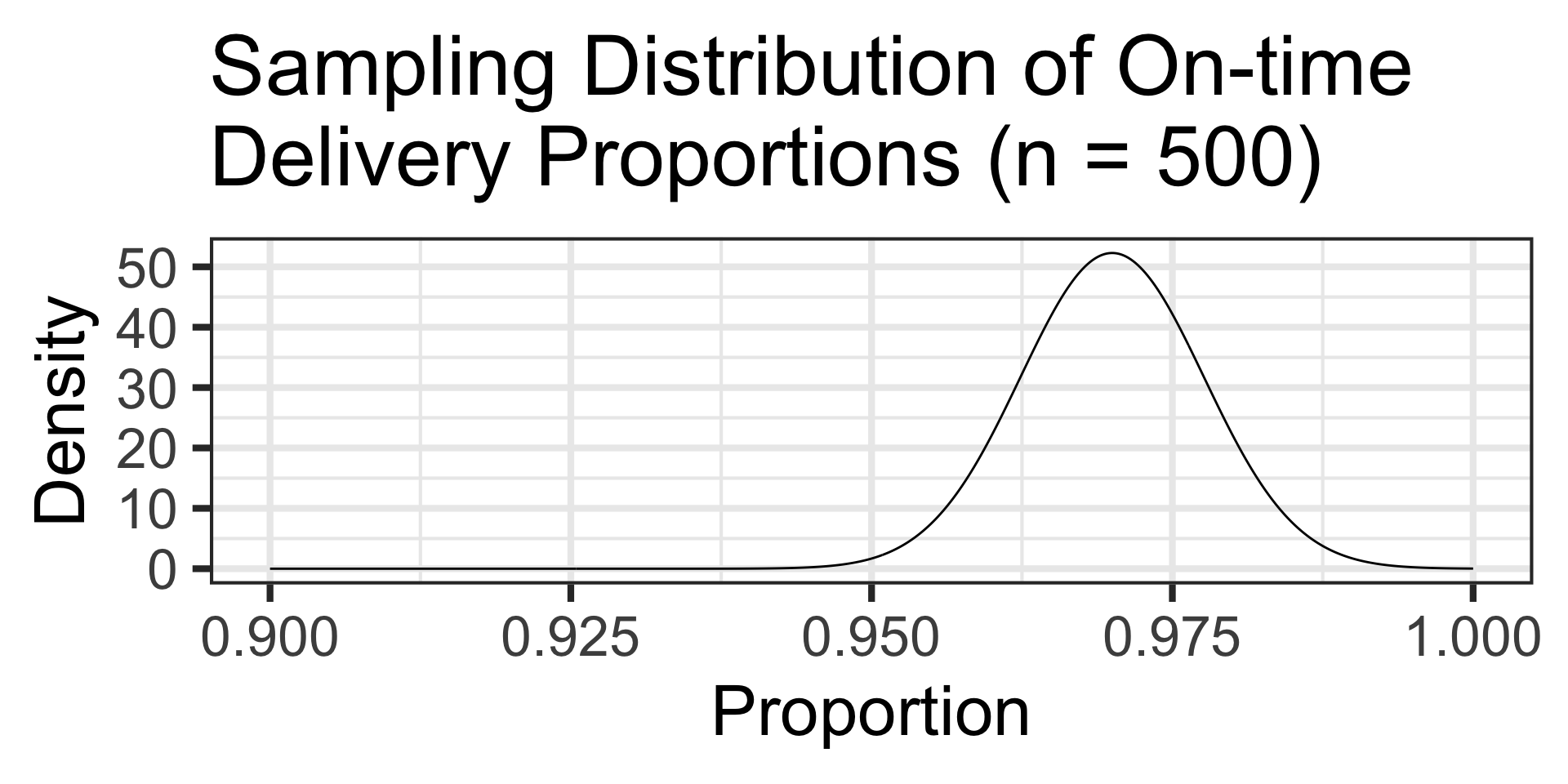
Completed Example: On-Time Package Delivery II

Scenario: A major online retailer, let’s call it “Amazonia”, has an internal benchmark to ensure that at least 97% of its packages are delivered on time. A logistics manager has concerns that a particular distribution center has been falling short of this target. The logistics manager takes a new random sample of 500 recent package deliveries. Out of these, 475 were delivered on time. Assuming that the facility is in compliance with the 97% on-time delivery rate, what is the probability that 95% or fewer packages arrive on time in a random sample of 500 deliveries.

Again the variable of interest is a proportion.
Since this is the case, we’ll check the success-failure condition…
$\begin{array}{lcl} n\cdot p & = & 500\cdot\left(0.97\right) = 485 \geq 10~\checkmark\\ n\cdot \left(1 - p\right) & = & 500\cdot\left(0.03\right) = 15 \geq 10~\checkmark \end{array}$
The success-failure condition is satisfied, so the CLT says that the sampling distribution for the proportion will be $\displaystyle{N\left(p,~S_E = \sqrt{\frac{p\left(1 - p\right)}{n}}\right)}$

Completed Example: On-Time Package Delivery II

Scenario: A major online retailer, let’s call it “Amazonia”, has an internal benchmark to ensure that at least 97% of its packages are delivered on time. A logistics manager has concerns that a particular distribution center has been falling short of this target. The logistics manager takes a new random sample of 500 recent package deliveries. Out of these, 475 were delivered on time. Assuming that the facility is in compliance with the 97% on-time delivery rate, what is the probability that 95% or fewer packages arrive on time in a random sample of 500 deliveries.

Again the variable of interest is a proportion.
Since this is the case, we’ll check the success-failure condition…
$\begin{array}{lcl} n\cdot p & = & 500\cdot\left(0.97\right) = 485 \geq 10~\checkmark\\ n\cdot \left(1 - p\right) & = & 500\cdot\left(0.03\right) = 15 \geq 10~\checkmark \end{array}$
The success-failure condition is satisfied, so the CLT
says that the sampling distribution for the proportion
will be $\displaystyle{N\left(p,~S_E = \sqrt{\frac{p\left(1 - p\right)}{n}}\right)}$

The probability of observing 95% or lower on-time package delivery proportions is…

Completed Example: On-Time Package Delivery II

Scenario: A major online retailer, let’s call it “Amazonia”, has an internal benchmark to ensure that at least 97% of its packages are delivered on time. A logistics manager has concerns that a particular distribution center has been falling short of this target. The logistics manager takes a new random sample of 500 recent package deliveries. Out of these, 475 were delivered on time. Assuming that the facility is in compliance with the 97% on-time delivery rate, what is the probability that 95% or fewer packages arrive on time in a random sample of 500 deliveries.

Again the variable of interest is a proportion.
Since this is the case, we’ll check the success-failure condition…
$\begin{array}{lcl} n\cdot p & = & 500\cdot\left(0.97\right) = 485 \geq 10~\checkmark\\ n\cdot \left(1 - p\right) & = & 500\cdot\left(0.03\right) = 15 \geq 10~\checkmark \end{array}$
The success-failure condition is satisfied, so the CLT
says that the sampling distribution for the proportion
will be $\displaystyle{N\left(p,~S_E = \sqrt{\frac{p\left(1 - p\right)}{n}}\right)}$

The probability of observing 95% or lower on-time package delivery proportions is…

S_E <- sqrt((0.97*0.03)/500)
pnorm(0.95, 0.97, S_E) $\approx$ 0.0044

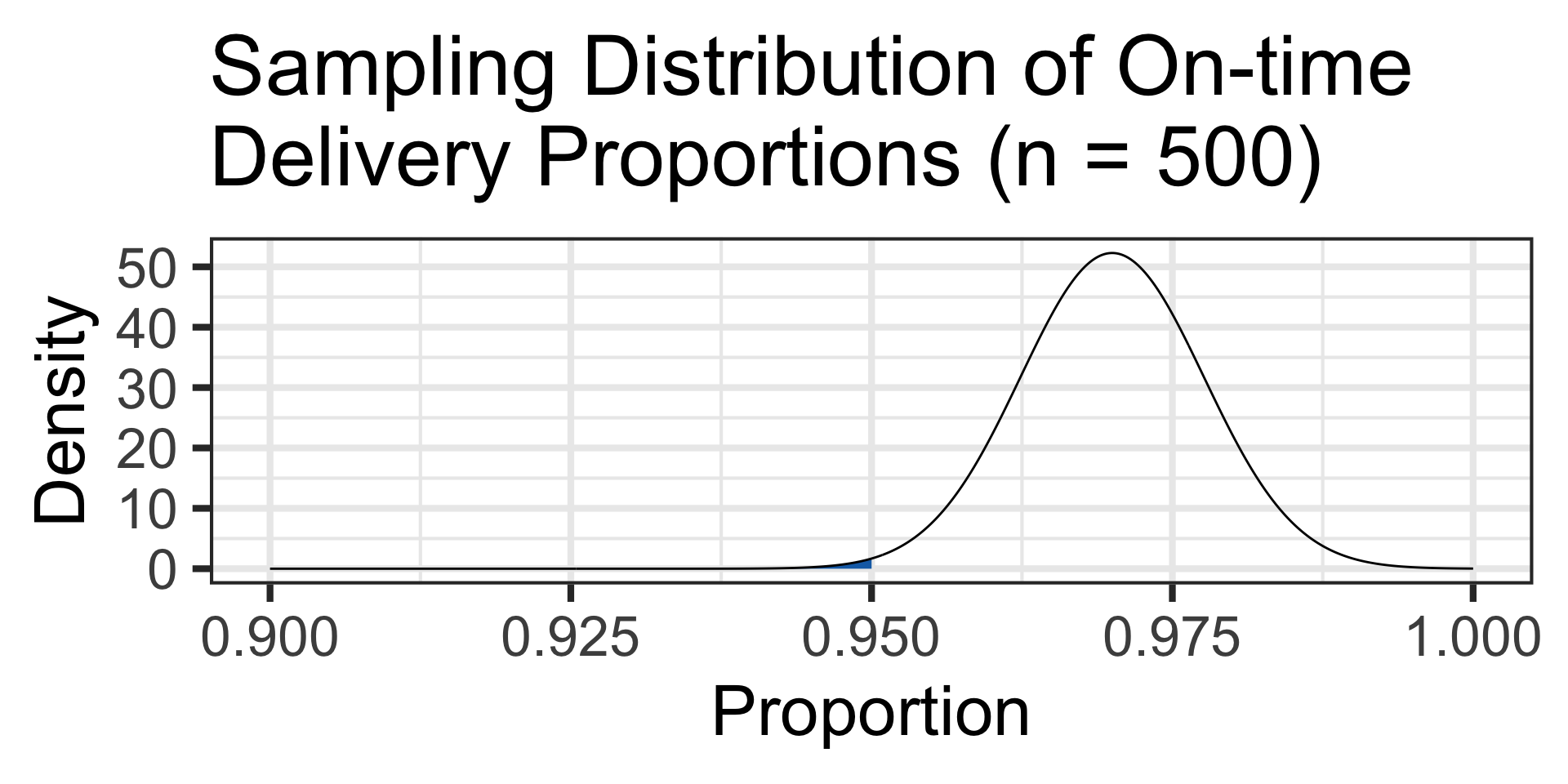
Completed Example: On-Time Package Delivery II

Scenario: A major online retailer, let’s call it “Amazonia”, has an internal benchmark to ensure that at least 97% of its packages are delivered on time. A logistics manager has concerns that a particular distribution center has been falling short of this target. The logistics manager takes a new random sample of 500 recent package deliveries. Out of these, 475 were delivered on time. Assuming that the facility is in compliance with the 97% on-time delivery rate, what is the probability that 95% or fewer packages arrive on time in a random sample of 500 deliveries.

Again the variable of interest is a proportion.
Since this is the case, we’ll check the success-failure condition…
$\begin{array}{lcl} n\cdot p & = & 500\cdot\left(0.97\right) = 485 \geq 10~\checkmark\\ n\cdot \left(1 - p\right) & = & 500\cdot\left(0.03\right) = 15 \geq 10~\checkmark \end{array}$
The success-failure condition is satisfied, so the CLT
says that the sampling distribution for the proportion
will be $\displaystyle{N\left(p,~S_E = \sqrt{\frac{p\left(1 - p\right)}{n}}\right)}$

The probability of observing 95% or lower on-time package delivery proportions is…

S_E <- sqrt((0.97*0.03)/500)
pnorm(0.95, 0.97, S_E) $\approx$ 0.0044

With such a low likelihood of observing only 95% on-time delivery, perhaps this distribution center is underperforming.

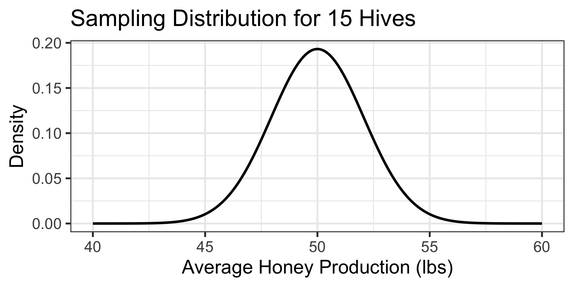
Completed Example: What’s the Buzz About Honey?

Senario: Beekeepers agree that the amount of honey collected from a typical hive over the summer is approximately normally distributed with a mean of 50 pounds and a standard deviation of 8 pounds. A beekeeper overseeing several locations monitors production at a particular site. At the end of the season, the beekeeper measures honey production from 15 randomly selected hives and observes an average of 47 pounds of honey per hive. What is the probability that a random sample of 15 hives would average 47 pounds or less of honey production?

The population distribution of honey production is approximately normal, so we can assume the sampling distribution will also be normal.
Honey production is a numerical variable, so the sampling distribution of the mean honey production from 15 hives is $\displaystyle{N\left(\mu, S_E = \sigma/\sqrt{n}\right)}$, which in this case is $\displaystyle{N\left(\mu = 50, S_E = 8/\sqrt{15}\right)}$.

Completed Example: What’s the Buzz About Honey?

Senario: Beekeepers have found that the amount of honey collected from a typical hive over the summer is approximately normally distributed with a mean of 50 pounds and a standard deviation of 8 pounds. A beekeeper overseeing several locations is monitoring their production at a particular site. At the end of the season, the beekeeper measures honey production from 15 randomly selected hives at that site and observes an average of 47 pounds of honey per hive. What is the probability that a random sample of 15 hives would average 47 pounds or less of honey production?

The population distribution of honey production is approximately normal, so we can assume the sampling distribution will also be normal.
Honey production is a numerical variable, so the sampling distribution of the mean honey production from 15 hives is $\displaystyle{N\left(\mu, S_E = \sigma/\sqrt{n}\right)}$, which in this case is $\displaystyle{N\left(\mu = 50, S_E = 8/\sqrt{15}\right)}$.

The probability of an average honey production of 47 pounds or less is…

Completed Example: What’s the Buzz About Honey?

Senario: Beekeepers have found that the amount of honey collected from a typical hive over the summer is approximately normally distributed with a mean of 50 pounds and a standard deviation of 8 pounds. A beekeeper overseeing several locations is monitoring their production at a particular site. At the end of the season, the beekeeper measures honey production from 15 randomly selected hives at that site and observes an average of 47 pounds of honey per hive. What is the probability that a random sample of 15 hives would average 47 pounds or less of honey production?

The population distribution of honey production is approximately normal, so we can assume the sampling distribution will also be normal.
Honey production is a numerical variable, so the sampling distribution of the mean honey production from 15 hives is $\displaystyle{N\left(\mu, S_E = \sigma/\sqrt{n}\right)}$, which in this case is $\displaystyle{N\left(\mu = 50, S_E = 8/\sqrt{15}\right)}$.

The probability of an average honey production of 47 pounds or less is…

pnorm(47, 50, 8/sqrt(15)) $\approx$ 0.0732

Completed Example: What’s the Buzz About Honey?

Senario: Beekeepers have found that the amount of honey collected from a typical hive over the summer is approximately normally distributed with a mean of 50 pounds and a standard deviation of 8 pounds. A beekeeper overseeing several locations is monitoring their production at a particular site. At the end of the season, the beekeeper measures honey production from 15 randomly selected hives at that site and observes an average of 47 pounds of honey per hive. What is the probability that a random sample of 15 hives would average 47 pounds or less of honey production?

The population distribution of honey production is approximately normal, so we can assume the sampling distribution will also be normal.
Honey production is a numerical variable, so the sampling distribution of the mean honey production from 15 hives is $\displaystyle{N\left(\mu, S_E = \sigma/\sqrt{n}\right)}$, which in this case is $\displaystyle{N\left(\mu = 50, S_E = 8/\sqrt{15}\right)}$.

The probability of an average honey production of 47 pounds or less is…

pnorm(47, 50, 8/sqrt(15)) $\approx$ 0.0732

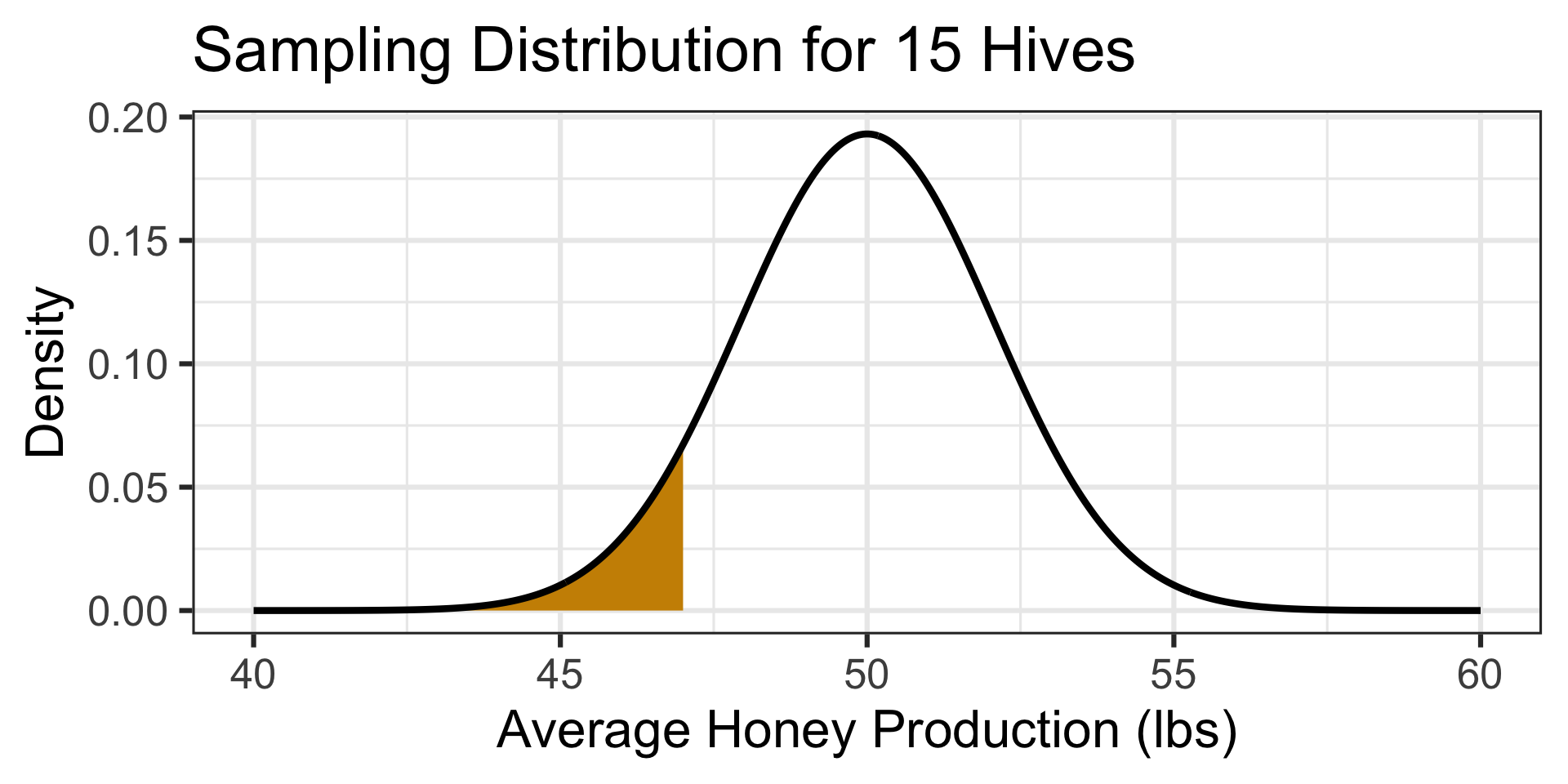
A 7.32% chance of observing a result as bad as they observed means that such an average is not totally unexpected, but they may want to investigate the environment around this site to see if there are abnormal conditions impacting honey production.

Examples to Try: Fast Food Waiting Times

Scenario: A popular fast-food chain claims that its wait time in its drive-thru is approximately normally distributed with a mean of 3.5 minutes and a standard deviation of 2.5 minutes. A consumer advocacy group randomly samples 40 customers from different locations, and the average wait time in the sample is 4 minutes. What is the probability of observing a random sample of 40 customers with an average wait time of at least 4 minutes?¹

Examples to Try: Mobile App Usage

Scenario: A mobile app company claims that 60% of its users open the app at least once a day. A marketing team conducts a survey, randomly sampling 200 users. Of those, 112 report using the app daily. What is the probability of observing a random sample of 200 users where less than 113 open the app at least once a day?¹

Examples to Try: Online Course Completion Rates

Scenario: An online education platform reports internally that 15% of students don’t complete their courses. A research team samples 120 students recently enrolled in a particular class, and 26 of them did not complete that course. What is the probability of observing a random sample of 120 students where 26 or more did not complete this course? What might this say about that course?¹

Examples to Try: Hospital Length of Stay

Scenario: A local hospital claims that the average length of stay for patients is 5.2 days, with a standard deviation of 2.1 days. A health department survey randomly samples 36 patients from recent discharges, and the average length of stay in the sample is 6.1 days. Find the probability of observing a random sample of 36 patients whose average stay length was at least 6.1 days. Assume that the population distribution of stay lengths is not strongly skewed.¹

Examples to Try: NFL Offensive Line, QB Protection

Scenario: In the NFL, one of the most important roles of the offensive line is to protect the quarterback from being sacked. The distribution of sacks per game is approximately normal. League-wide, teams allow an average of 2.3 sacks per game, with a standard deviation of 0.9 sacks. The coaching staff of a particular team believes their offensive line is better than average. Over the course of 17 games in the regular season, they allow an average of 1.8 sacks per game. What is the probability that a random sample of 17 games would result in an average of 1.8 sacks or fewer?¹

Summary and Next Time…

The sampling distribution is a theoretical distribution of sample statistics (ie. sample means or sample proportions) coming from samples of a common size
As long as sample sizes are large enough, the sampling distribution is nearly normal
- For means, “large enough” is having enough observations in the sample to overcome skew in the population distribution – more skew means larger samples are necessary
- For proportions, “large enough” means that the success-failure condition is satisfied – the sample size is large enough that we “expect” at least 10 successes and at least 10 failures
The Central Limit Theorem tells us that the normal distributions approximating our sampling distribution are:
- For sample means: $\displaystyle{N\left(\mu, S_E = \sigma/\sqrt{n}\right)}$
- For sample proportions: $\displaystyle{N\left(p, S_E = \sqrt{\frac{p\left(1 - p\right)}{n}}\right)}$
When sample sizes are large enough (as described above), we can use pnorm() to calculate probabilities associated with outcomes from samples, using the appropriate sampling distribution

Next Time:

Inference on Categorical Data