02:00
Discrete Probability: The Binomial Distribution
Dr. Gilbert
January 2, 2026
The Highlights
- Computing with R: Warmup Problems
- A very quick review
- Binomial Experiments
- The Binomial Distribution
- Expected Value and Standard Deviation
- Examples: Binomial or Not?
- Review of R functionality for probabilities and the Binomial Distribution
pbinom()dbinom()
- Examples: Calculating Probabilities
Computing with R
We’ve been focused on working with data frames recently
Let’s remember how to use R for basic calculations
Example: Consider the small data set: 54, 98, 72, 81, 89, 85, 78, 84. Use R functionality to compute each of the following.
- the mean
- the median
- the standard deviation
- the interquartile range
A Note on this Deck
This slide deck contains a detailed overview of binomial experiments and the binomial distribution.
We’ll run through these very quickly during our in-class discussion since you’ve already spent time learning about these foundational ideas in the interactive notebook.
If you have questions about the definitions of binomial experiments or the binomial distribution during or after our discussions of these example problems, refer back to these review slides and visit me in office hours.
Binomial Experiments
A binomial experiment is a statistical experiment that:
- Consists of a fixed number of independent trials
- Each trial has two possible outcomes, often called success or failure for convenience
- The probability of success is the same for each trial
The key characteristics to identify are:
- The number of trials, \(n\)
- The outcomes – What is meant by success? What is meant by failure?
- The probability of success, \(p\)
- The number of successes we are interested in, \(k\)
The Binomial Distribution
The number of successes in a binomial experiment is a random variable, \(X\)
The number of successful outcomes, \(X\), follows a binomial distribution with parameters \(n\) (trials) and \(p\) (success probability) and we write
\[X \sim \text{Binomial}\left(n, p\right)\]
Mathematically, the probability of observing exactly \(k\) successes out of \(n\) trials in a binomial experiment with success probability \(p\) is given by
\[\mathbb{P}\left[X = k\right] = \binom{n}{k} p^k \left(1 - p\right)^{n - k}\]
Where \(\displaystyle{\binom{n}{k} = \frac{n!}{k!\left(n -k\right)!}}\) is the number of ways to choose the \(k\) successful trials out of the \(n\) total trials
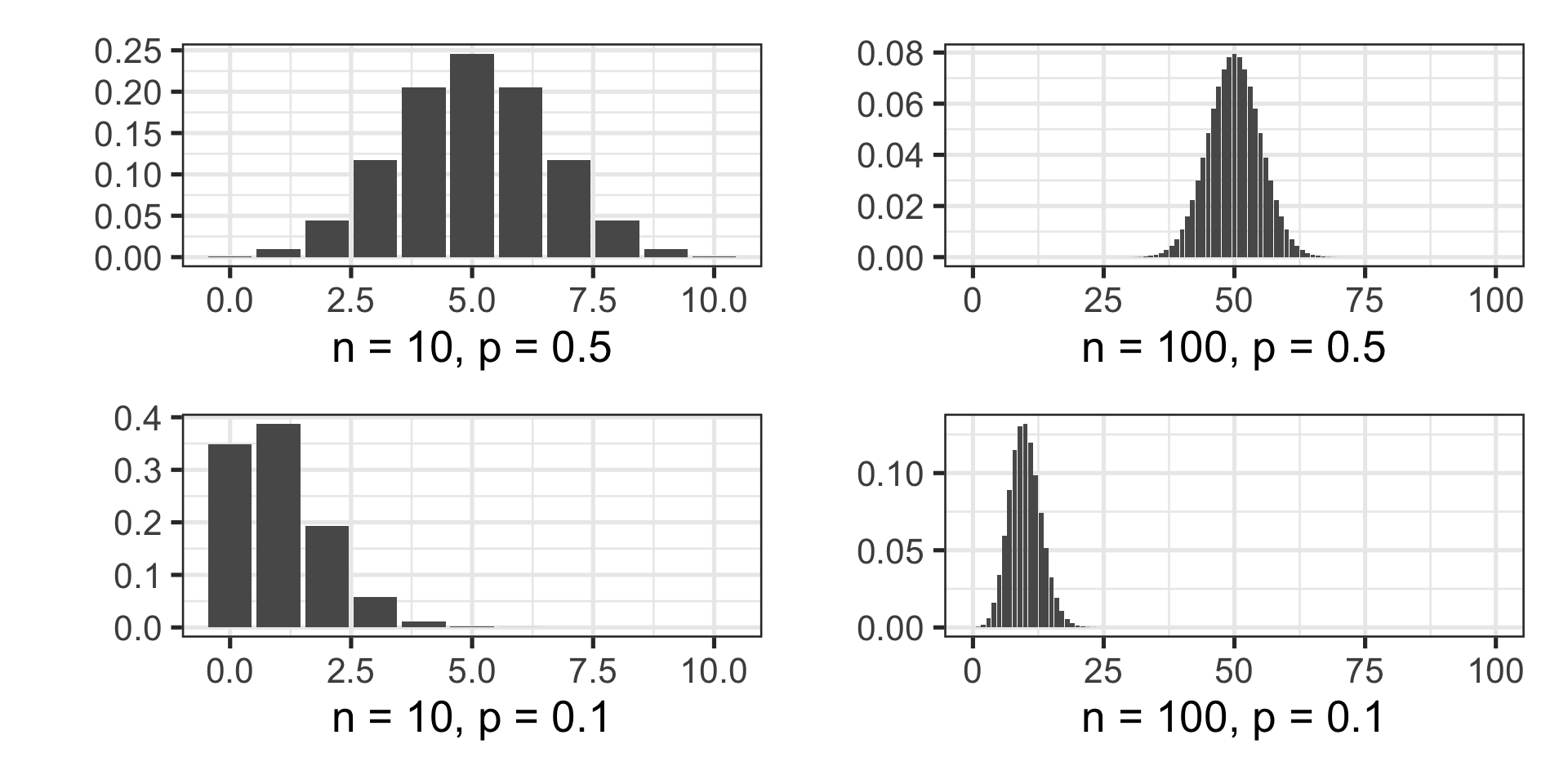
The Binomial Distribution
\[\mathbb{P}\left[X = k\right] = \binom{n}{k}\cdot p^k\cdot\left(1 - p\right)^{n - k}\]
Below are examples of binomial distributions
Expected Value and Standard Deviation
On the previous slide, we saw that the center and spread of the binomial distribution depend on the values of \(n\) and \(p\)
Expected Value (mean/center): For a binomial distribution with \(n\) trials and success probability \(p\), the expected number of successes, \(\mathbb{E}\left[X\right]\), is \(n\cdot p\)
- For example, the binomial distribution with success probability 0.5 and 100 trials (the top-right plot on the previous slide), the expected number of successes is \(\mathbb{E}\left[X\right] = 100\cdot\left(0.5\right) = 50\)
\(\bigstar\) Try It! Find the expected number of successes in a binomial experiment with 50 trials and probability of success 0.25.
00:30
Expected Value and Standard Deviation
On the previous slide, we saw that the center and spread of the binomial distribution depend on the values of \(n\) and \(p\)
Standard Deviation (spread): For a binomial distribution with \(n\) trials and success probability \(p\), the standard deviation of the number of successes, \(\text{sd}\left(X\right)\), is \(\sqrt{n\cdot p\cdot\left(1 - p\right)}\)
- Again, for example, the binomial distribution with success probability 0.5 and 100 trials (the top-right plot on the previous slide), the standard deviation in the number of successes is \(\text{sd}\left(X\right) = \sqrt{100\cdot\left(0.5\right)\cdot\left(1 - 0.5\right)} = 5\)
\(\bigstar\) Try It! Find the standard deviation in number of successes in a binomial experiment with 50 trials and probability of success 0.25.
00:30
Example Problems: Binomial or Not?
For each of the following example scenarios, determine whether they can be modeled as binomial experiments or not.
Scenario: It is estimated that 77% of people have been in at least one car accident in their lives. Researchers asked 48 randomly selected individuals whether they have ever been in a car accident.
00:30
Example Problems: Binomial or Not?
For each of the following example scenarios, determine whether they can be modeled as binomial experiments or not.
Scenario: A researcher surveys students one by one, asking if they agree with a policy. The researcher continues until exactly 50 students say they agree with the policy.
00:30
Example Problems: Binomial or Not?
For each of the following example scenarios, determine whether they can be modeled as binomial experiments or not.
Scenario: You are measuring the time until a machine fails. Each machine’s lifespan is recorded, but failures occur at unpredictable times based on complex factors such as wear and tear.
00:30
Example Problems: Binomial or Not?
For each of the following example scenarios, determine whether they can be modeled as binomial experiments or not.
Scenario: A factory has a defect rate of 3% in the products it manufactures. Inspectors randomly select and evaluate 100 products.
00:30
Example Problems: Binomial or Not?
For each of the following example scenarios, determine whether they can be modeled as binomial experiments or not.
Scenario: A botanist finds that a certain species of plant successfully grows 60% of the time under controlled greenhouse conditions. The botanist plants 25 seeds.
00:30
Example Problems: Binomial or Not?
For each of the following example scenarios, determine whether they can be modeled as binomial experiments or not.
Scenario: In a classroom, groups of 5 students vote on whether to select a particular project topic. We count the number of “yes” votes. The students in the group discuss the topic before voting.
00:30
Ask Me Two Questions
Before we move forward, ask me two questions…
Calculating Probabilities with the Binomial Distribution
As a reminder, the binomial distribution for \(n\) trials and a success probability \(p\) is given by
\[\mathbb{P}\left[X = k\right] = \binom{n}{k}\cdot p^k\cdot\left(1 - p\right)^{n - k}\]
We have two helper-functions in R that we can use to compute probabilities using the binomial distribution without manually evaluating this formula.
- \(\mathbb{P}\left[X = k\right] \approx \text{dbinom}\left(k, n, p\right)\)
\[X~\text{(successes)}:~0,~1,~2,~\cdots,~k - 1,~\color{blue}{\boxed{k}},~k+1,~\cdots,~n - 1, n\]
- \(\mathbb{P}\left[X \leq k\right] \approx \text{pbinom}\left(k, n, p\right)\)
\[X~\text{(successes)}:~\color{blue}{\boxed{0,~1,~2,~\cdots,~k - 1,~k}},~k+1,~\cdots,~n - 1, n\]
On Drawing Pictures: Drawing pictures, like those above, to model problems in statistics is probably the best favor that you can do for yourself. Students who commit to drawing pictures early on never regret it.
A Completed Example (Part I)
Example: It is estimated that 77% of people have been in at least one car accident in their lives. Researchers asked 48 randomly selected individuals whether they have ever been in a car accident.
- Find the probability that exactly 40 of the individuals have been in at least one car accident.
Notice that \(n = 48\), \(p = 0.77\), and \(k = 40\).
Draw a Picture: It really helps…
\[X~\text{(successes)}:~0,~1,~2,~\cdots,~39,~40,~41,~\cdots,~48\]
A Completed Example (Part I)
Example: It is estimated that 77% of people have been in at least one car accident in their lives. Researchers asked 48 randomly selected individuals whether they have ever been in a car accident.
- Find the probability that exactly 40 of the individuals have been in at least one car accident.
Notice that \(n = 48\), \(p = 0.77\), and \(k = 40\).
Draw a Picture: It really helps…
\[X~\text{(successes)}:~0,~1,~2,~\cdots,~39,~\color{blue}{~\boxed{40}~},~41,~\cdots,~48\]
A Completed Example (Part II)
Example: It is estimated that 77% of people have been in at least one car accident in their lives. Researchers asked 48 randomly selected individuals whether they have ever been in a car accident.
- Find the probability at most 30 of the individuals have been in at least one car accident.
Notice that \(n = 48\), \(p = 0.77\), and \(k = 30\).
Draw a Picture: It really helps…
\[X~\text{(successes)}:~0,~1,~2,~\cdots,~29,~30,~31,~\cdots,~48\]
A Completed Example (Part II)
Example: It is estimated that 77% of people have been in at least one car accident in their lives. Researchers asked 48 randomly selected individuals whether they have ever been in a car accident.
- Find the probability at most 30 of the individuals have been in at least one car accident.
Notice that \(n = 48\), \(p = 0.77\), and \(k = 30\).
Draw a Picture: It really helps…
\[X~\text{(successes)}:~\color{blue}{\boxed{~0,~1,~2,~\cdots,~29,~30~}},~31,~\cdots,~48\]
A Completed Example (Part III)
Example: It is estimated that 77% of people have been in at least one car accident in their lives. Researchers asked 48 randomly selected individuals whether they have ever been in a car accident.
- Find the probability that more than 35 of the individuals have been in at least one car accident.
Notice that \(n = 48\), \(p = 0.77\), and \(k = ??\).
Draw a Picture: It really helps…
\[X~\text{(successes)}:~0,~1,~2,~\cdots,~34,~35,~36,~\cdots,~48\]
A Completed Example (Part III)
Example: It is estimated that 77% of people have been in at least one car accident in their lives. Researchers asked 48 randomly selected individuals whether they have ever been in a car accident.
- Find the probability that more than 35 of the individuals have been in at least one car accident.
Notice that \(n = 48\), \(p = 0.77\), and \(k = ??\).
Draw a Picture: It really helps…
\[X~\text{(successes)}:~0,~1,~2,~\cdots,~34,~35,~\color{blue}{\boxed{~36,~\cdots,~48~}}\]
A Completed Example (Part III)
Example: It is estimated that 77% of people have been in at least one car accident in their lives. Researchers asked 48 randomly selected individuals whether they have ever been in a car accident.
- Find the probability that more than 35 of the individuals have been in at least one car accident.
Notice that \(n = 48\), \(p = 0.77\), and \(k = ??\).
Draw a Picture: It really helps…
\[X~\text{(successes)}:~\color{red}{\boxed{~0,~1,~2,~\cdots,~34,~35~}},~\color{blue}{\boxed{~36,~\cdots,~48~}}\]
A Completed Example (Part III)
Example: It is estimated that 77% of people have been in at least one car accident in their lives. Researchers asked 48 randomly selected individuals whether they have ever been in a car accident.
- Find the probability that more than 35 of the individuals have been in at least one car accident.
Notice that \(n = 48\), \(p = 0.77\), and \(k = ??\).
Draw a Picture: It really helps…
\[X~\text{(successes)}:~\color{black}{~\boxed{\color{red}{\boxed{~0,~1,~2,~\cdots,~34,~35~}},~\color{blue}{\boxed{~36,~\cdots,~48~}}~}}\]
We should start with “everything” (a probability of 1) and remove the probability that at most 35 individuals have been in at least one car accident.
A Completed Example (Part III)
Example: It is estimated that 77% of people have been in at least one car accident in their lives. Researchers asked 48 randomly selected individuals whether they have ever been in a car accident.
- Find the probability that more than 35 of the individuals have been in at least one car accident.
Notice that \(n = 48\), \(p = 0.77\), and \(k = ??\).
Draw a Picture: It really helps…
\[X~\text{(successes)}:~\color{black}{~\boxed{~\color{red}{\boxed{~0,~1,~2,~\cdots,~34,~35~}},~\color{blue}{\boxed{~36,~\cdots,~48~}}~}}\]
A Completed Example (Part IV)
Example: It is estimated that 77% of people have been in at least one car accident in their lives. Researchers asked 48 randomly selected individuals whether they have ever been in a car accident.
- Find the probability that at least 35 but less than 42 of the individuals have been in at least one car accident.
Notice that \(n = 48\), \(p = 0.77\), and \(k = ??\).
Draw a Picture: It really helps…
\[X~\text{(successes)}:~0,~1,~2,~\cdots,~34,~35,~36,~\cdots,~41,~42,~43,~\cdots,~48~\]
A Completed Example (Part IV)
Example: It is estimated that 77% of people have been in at least one car accident in their lives. Researchers asked 48 randomly selected individuals whether they have ever been in a car accident.
- Find the probability that at least 35 but less than 42 of the individuals have been in at least one car accident.
Notice that \(n = 48\), \(p = 0.77\), and \(k = ??\).
Draw a Picture: It really helps…
\[X~\text{(successes)}:~\color{black}{\boxed{~0,~1,~2,~\cdots,~34,~35,~36,~\cdots,~41}},~42,~43,~\cdots,~48~\]
A Completed Example (Part IV)
Example: It is estimated that 77% of people have been in at least one car accident in their lives. Researchers asked 48 randomly selected individuals whether they have ever been in a car accident.
- Find the probability that at least 35 but less than 42 of the individuals have been in at least one car accident.
Notice that \(n = 48\), \(p = 0.77\), and \(k = ??\).
Draw a Picture: It really helps…
\[X~\text{(successes)}:~\color{black}{\boxed{~0,~1,~2,~\cdots,~34,~\color{blue}{\boxed{~35,~36,~\cdots,~41}~}~}},~42,~43,~\cdots,~48~\]
A Completed Example (Part IV)
Example: It is estimated that 77% of people have been in at least one car accident in their lives. Researchers asked 48 randomly selected individuals whether they have ever been in a car accident.
- Find the probability that at least 35 but less than 42 of the individuals have been in at least one car accident.
Notice that \(n = 48\), \(p = 0.77\), and \(k = ??\).
Draw a Picture: It really helps…
\[X~\text{(successes)}:~\color{black}{\boxed{\color{red}{\boxed{~0,~1,~2,~\cdots,~34~}},~\color{blue}{\boxed{~35,~36,~\cdots,~41}~}~}},~42,~43,~\cdots,~48~\]
We should start with the probability that at most 41 individuals have been in at least one car accident and then remove the probability that at most 34 individuals have been in at least one car accident.
Try It, Example 1
Scenario: A factory has a defect rate of 3% in the products it manufactures. Inspectors randomly select 100 products.
- What is the probability that exactly 5 products have defects?
- What is the probability that at most 5 products have defects?
- What is the probability that at least 5 products have defects?
Try It, Example 2
Scenario: A botanist finds that a certain species of plant successfully grows 60% of the time under controlled greenhouse conditions. The botanist plants 25 seeds.
- What is the probability that exactly 20 of the seeds grow?
- What is the probability that fewer than 20 of the seeds grow?
- What is the probability that at least 17 and no more than 21 of the seeds grow?
- What is the probability that more than 20 of the seeds grow?
Exit Ticket Task
Navigate to our MAT241 Exit Ticket Form, answer the questions, and complete the task below.
Note. Today’s discussion is listed as 1. Intro to Data

Task: Describe your approach and answers to the following questions. A package delivery company experiences delays randomly with probability 1.5%. That is, there is a 1.5% chance that a randomly selected package is delayed. A random sample of 500 package deliveries from the company is examined. What is the probability that 15 or more are delayed? What does this suggest?
Summary
- Binomial Experiments involve a fixed number of independent trials (\(n\)), two possible outcomes for each trial, and a constant probability of “success” (\(p\)).
- The Binomial Distribution is a probability distribution over the number of successful outcomes in these experiments.
- We can calculate probabilities associated with counts of successful outcomes using the binomial distribution \(\displaystyle{\mathbb{P}\left[X = k\right] = \binom{n}{k}\cdot p^k\cdot\left(1 - p\right)^{n - k}}\).
- We can also use R functionality to avoid having to compute this by hand!
- \(\mathbb{P}\left[X = k\right] \approx \text{dbinom}\left(k, n, p\right)\)
- \(\mathbb{P}\left[X \leq k\right] \approx \text{pbinom}\left(k, n, p\right)\)
- Don’t try to memorize how to apply this functionality in different scenarios – just draw pictures and use the picture to guide you.
Next Time…
The Normal Distribution