Introduction to Logistic Regression
Purpose: In this notebook, we introduce the class of model known as logistic regression. In particular, we note the following.
- Polynomial regression models cannot be used for classification since they are unbounded.
- Logistic regression models take the form \(\displaystyle{\mathbb{P}\left[y = 1\right] = \frac{e^{\beta_0 + \beta_1x_1 + \cdots + \beta_kx_k}}{1 + e^{\beta_0 + \beta_1x_1 + \cdots + \beta_kx_k}}}\)
- The output of a logistic regression model \(\mathbb{P}\left[y = 1\right]\) is the predicted probability that the corresponding observation belongs to the class labeled by 1.
- The output of a logistic regression model is bounded between \(0\) and \(1\).
Toy Data
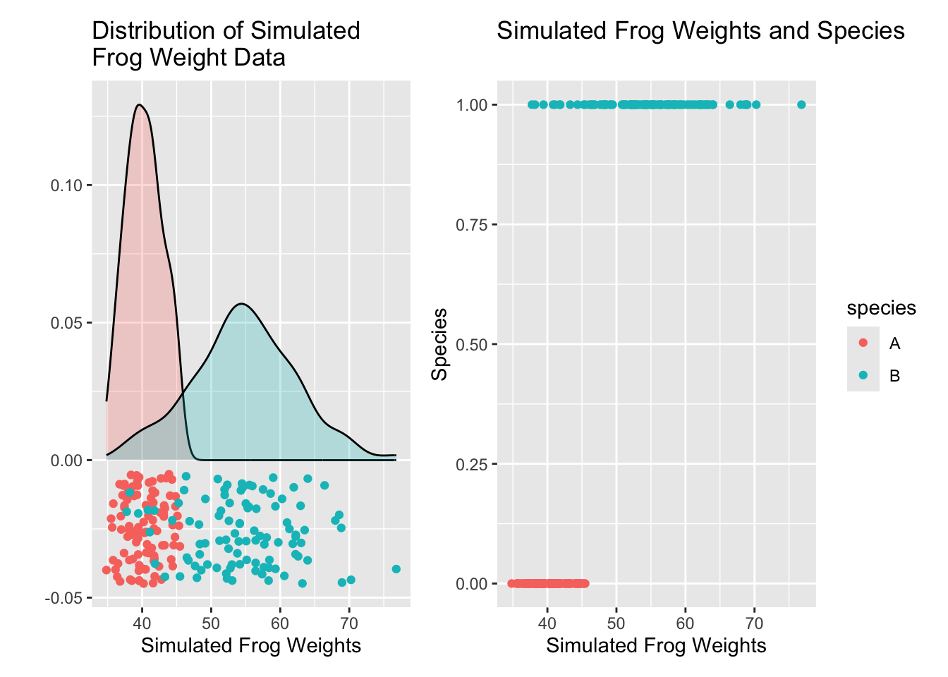
In order to have an example to work with, we’ll develop a toy dataset. Let’s say that we are able to weights of two species of frog, and that the weights are normally distributed in each population. The weights in Species A follow \(W_A \sim N\left(\mu = 40, \sigma = 3\right)\) and the weights in Species B follow \(W_B \sim N\left(\mu = 55, \sigma = 7\right)\).
We’ll simulate drawing \(100\) frogs from each population and recording their weights. The results appear below. Note that in the plot on the left, the vertical position of the observed data points is meaningless – some noise has been added so that the observed frog weights are discernible from one another.
Our goal then is to fit a model that will help us determine whether a frog with a given weight is most likely to belong to Species A or Species B.
Why Not Linear Regression?
Linear regression techniques are problematic here because of the nature of polynomial functions. They are [nearly] all unbounded – that is, eventually, any non-constant polynomial will escape the interval \(\left[0, 1\right]\) and predicted values will run off towards positive or negative infinity. You can see this below where we are fitting and plotting several linear regression models to the simulated frog weight data.
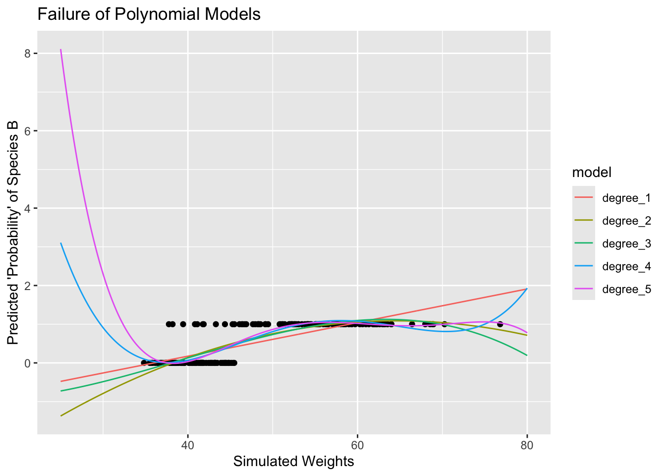
Note that these polynomial-form linear regression models all eventually escape the \(\left[0, 1\right]\) interval. The outputs from these models cannot be interpreted as probabilities.
Logistic Regression
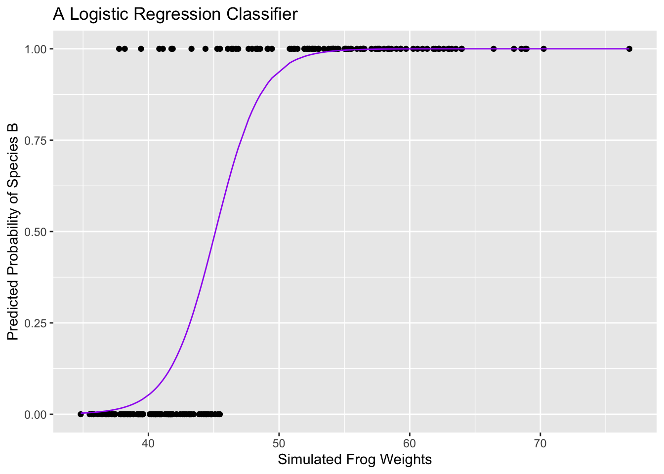
A logistic regression model takes the form \(\displaystyle{\mathbb{P}\left[y = 1\right] = \frac{e^{\beta_0 + \beta_1x_1 + \cdots + \beta_kx_k}}{1 + e^{\beta_0 + \beta_1x_1 + \cdots + \beta_kx_k}}}\). The outputs from such a model are bounded to the interval \(\left[0, 1\right]\). As a result, we can interpret the outputs from such a model as the probability that an observation belongs to the class labeled by 1.
Below we fit and plot a logistic regression model.
Properties
Logistic regression models are linear models since we can show that an equivalent form for the model is \[\log\left(\frac{p}{1 - p}\right) = \beta_0 + \beta_1x_1 + \cdots + \beta_kx_k\]
This means that the decision boundary for a logistic regression model corresponds to the situation where \(p = 1 - p\) (or \(p = 0.5\)). This would result in the equation \(\beta_0 + \beta_1x_1 + \cdots + \beta_kx_k = 0\), a line/plane/hyperplane.
Interpretations and Marginal Effects
Since the linear form of a logistic regression model outputs the log-odds of belonging to the class labeled by 1 and not the probability of belonging to that class, it can be difficult to interpret logistic regression models. In particular,
If \(x_i\) is a numeric predictor, then \(\beta_i\) is the expected impact on the log-odds of an observation belonging to the class labeled by 1 due to a unit increase in \(x_i\).
- Note that this is not the same as the effect on the probability of an observation belonging to the class labeled by 1.
In order to obtain the expected effect of a unit increase in \(x_i\) on the probability of an observation belonging to the class labeled by 1, we would need to compute the partial derivative of the original form of our logistic regression model with respect to \(x_i\). Multivariable calculus helps with this, but so does the
{marginaleffects}package.
| term | estimate | std.error | statistic | p.value |
|---|---|---|---|---|
| (Intercept) | -25.4802018 | 4.0467529 | -6.296456 | 0 |
| weight | 0.5646207 | 0.0920456 | 6.134142 | 0 |
The estimate attached to weight in the table above is the estimated increase in log-odds of belonging to Species B. This is difficult to interpret other than to say that heavier frogs are more likely to belong to Species B because the coefficient on weight is positive. We can use the slopes() function from the {marginaleffects} to compute the partial derivative of the logistic regression model with respect to weight at various levels of the weight variable.
| term | weight | estimate | conf.low | conf.high | std.error |
|---|---|---|---|---|---|
| weight | 40.25424 | 0.0318365 | 0.0143582 | 0.0493147 | 0.0089176 |
| weight | 41.27119 | 0.0516167 | 0.0286864 | 0.0745470 | 0.0116993 |
| weight | 42.28814 | 0.0787331 | 0.0479442 | 0.1095220 | 0.0157089 |
| weight | 43.30508 | 0.1095022 | 0.0680970 | 0.1509074 | 0.0211255 |
| weight | 44.32203 | 0.1340925 | 0.0857860 | 0.1823990 | 0.0246466 |
| weight | 45.33898 | 0.1406556 | 0.0977008 | 0.1836103 | 0.0219161 |
| weight | 46.35593 | 0.1254641 | 0.0940361 | 0.1568922 | 0.0160350 |
| weight | 47.37288 | 0.0967890 | 0.0665290 | 0.1270490 | 0.0154390 |
| weight | 48.38983 | 0.0666944 | 0.0342162 | 0.0991726 | 0.0165708 |
| weight | 49.40678 | 0.0424878 | 0.0129806 | 0.0719950 | 0.0150550 |
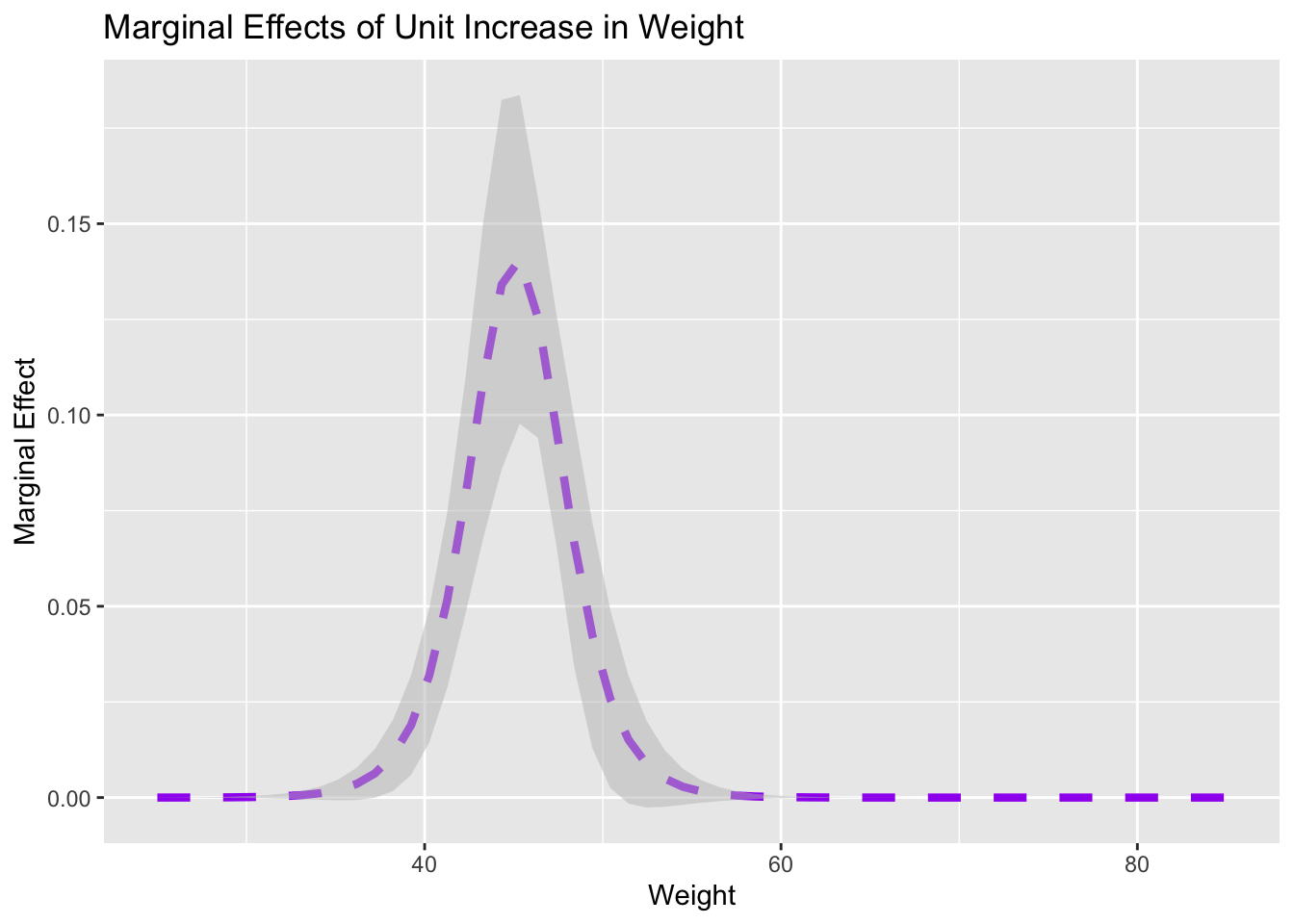
The output above shows estimates for the marginal effects of a unit increase in weight. We can see that the marginal effect is largest near a weight of about 45 units. For weights less than 35 units and more than 55 units, there is little change in probability that the corresponding observation belongs to Species B. Plots like the one above can be really helpful in understanding what our model suggests is the association between our predictor(s) and response.
How to Implement in {tidymodels}
A logistic regressor is a model class (that is, a model specification). We define our intention to build a logistic regressor using
log_reg_spec <- logistic_reg() %>%
  set_engine("glm") %>%
  set_mode("classification")
Hyperparameters and Other Extras
The lines to set_engine() and set_mode() are unnecessary since these are the defaults. I include them here just so that we continue to be reminded that setting an engine and setting a mode are typically things that we will need to do.
Depending on the fitting engine chosen, logistic regression models have two (2) tunable hyperparameters. They are
penalty, which is a model constraint penalizing the inclusion of multiple model terms and large coefficients.- Typical penalty values are powers of 10 – for example
1e-3, 0.01, 0.1, 1, 10. - Remember to scale all of your numerical predictors if you use this parameter. Otherwise some predictors are artificially cheap or expensive depending on the magnitude of their raw values.
- Typical penalty values are powers of 10 – for example
mixtureis a number between \(0\) and \(1\) which determines the type of regularization to use. Basically, this governs how our “spent coefficient budget is computed”.mixture = 0results inL1regularization (Ridge Regression)mixture = 1results inL2regularization (LASSO)mixturevalues between \(0\) and \(1\) are a mixture of Ridge and LASSO, where the value provided represents the proportion of the budget calculation corresponding to the LASSO.- As a reminder, you can read more about Ridge Regression, the LASSO, and how these approaches work here.
You can see the full {parsnip} documentation for logistic_reg() here.
Summary
In this notebook, we were introduced to the class of logistic regression models for classification. Logistic regressors are a sort of hybrid regression/classification model because they output a numerical values – interpreted as the probability that an observation belongs to the class labeled by 1. We saw two different forms for logistic regression models and we saw how we can interpret logistic regression models. In particular, we saw how we can use the {marginaleffects} package to help us understand what our model tells us about the association between predictor(s) and our response.