Purpose: The previous two notebooks have discussed theoretical and foundational aspects of deep learning models. In particular, what types of architectures and activation functions exist (and, to a lesser extent, how do I choose one). In this notebook our goal will be to actually build, assess, and utilize a deep learning network for image classification.
Data and Modeling
Since you set up TensorFlow in an earlier notebook, let’s load the {tidyverse}, {tensorflow}, {keras}, and {reticulate} libraries and get some data. We’ll use the Fashion MNIST data set. You can learn more about that data set from its official repository here .
library (tidyverse)library (tensorflow)library (keras)library (reticulate)use_virtualenv ("r-reticulate" )c (c (x_train, y_train), c (x_test, y_test)) %<-% keras:: dataset_fashion_mnist ()
Downloading data from https://storage.googleapis.com/tensorflow/tf-keras-datasets/train-labels-idx1-ubyte.gz
8192/29515 [=======>......................] - ETA: 0s������������������������������������������������������
29515/29515 [==============================] - 0s 1us/step
Downloading data from https://storage.googleapis.com/tensorflow/tf-keras-datasets/train-images-idx3-ubyte.gz
8192/26421880 [..............................] - ETA: 0s������������������������������������������������������������
139264/26421880 [..............................] - ETA: 9s������������������������������������������������������������
589824/26421880 [..............................] - ETA: 4s������������������������������������������������������������
1032192/26421880 [>.............................] - ETA: 4s������������������������������������������������������������
1654784/26421880 [>.............................] - ETA: 3s������������������������������������������������������������
2523136/26421880 [=>............................] - ETA: 2s������������������������������������������������������������
3080192/26421880 [==>...........................] - ETA: 2s������������������������������������������������������������
3653632/26421880 [===>..........................] - ETA: 2s������������������������������������������������������������
4227072/26421880 [===>..........................] - ETA: 2s������������������������������������������������������������
4784128/26421880 [====>.........................] - ETA: 2s������������������������������������������������������������
5341184/26421880 [=====>........................] - ETA: 2s������������������������������������������������������������
5906432/26421880 [=====>........................] - ETA: 2s������������������������������������������������������������
6447104/26421880 [======>.......................] - ETA: 1s������������������������������������������������������������
6995968/26421880 [======>.......................] - ETA: 1s������������������������������������������������������������
7585792/26421880 [=======>......................] - ETA: 1s������������������������������������������������������������
8134656/26421880 [========>.....................] - ETA: 1s������������������������������������������������������������
8683520/26421880 [========>.....................] - ETA: 1s������������������������������������������������������������
9011200/26421880 [=========>....................] - ETA: 1s������������������������������������������������������������
9625600/26421880 [=========>....................] - ETA: 1s������������������������������������������������������������
10182656/26421880 [==========>...................] - ETA: 1s������������������������������������������������������������
10731520/26421880 [===========>..................] - ETA: 1s������������������������������������������������������������
11280384/26421880 [===========>..................] - ETA: 1s������������������������������������������������������������
11829248/26421880 [============>.................] - ETA: 1s������������������������������������������������������������
12386304/26421880 [=============>................] - ETA: 1s������������������������������������������������������������
12943360/26421880 [=============>................] - ETA: 1s������������������������������������������������������������
13500416/26421880 [==============>...............] - ETA: 1s������������������������������������������������������������
14082048/26421880 [==============>...............] - ETA: 1s������������������������������������������������������������
14630912/26421880 [===============>..............] - ETA: 1s������������������������������������������������������������
15204352/26421880 [================>.............] - ETA: 1s������������������������������������������������������������
15777792/26421880 [================>.............] - ETA: 1s������������������������������������������������������������
15908864/26421880 [=================>............] - ETA: 1s������������������������������������������������������������
16908288/26421880 [==================>...........] - ETA: 0s������������������������������������������������������������
17448960/26421880 [==================>...........] - ETA: 0s������������������������������������������������������������
18022400/26421880 [===================>..........] - ETA: 0s������������������������������������������������������������
18595840/26421880 [====================>.........] - ETA: 0s������������������������������������������������������������
19152896/26421880 [====================>.........] - ETA: 0s������������������������������������������������������������
19726336/26421880 [=====================>........] - ETA: 0s������������������������������������������������������������
20299776/26421880 [======================>.......] - ETA: 0s������������������������������������������������������������
20865024/26421880 [======================>.......] - ETA: 0s������������������������������������������������������������
21413888/26421880 [=======================>......] - ETA: 0s������������������������������������������������������������
21987328/26421880 [=======================>......] - ETA: 0s������������������������������������������������������������
22544384/26421880 [========================>.....] - ETA: 0s������������������������������������������������������������
23134208/26421880 [=========================>....] - ETA: 0s������������������������������������������������������������
23707648/26421880 [=========================>....] - ETA: 0s������������������������������������������������������������
24281088/26421880 [==========================>...] - ETA: 0s������������������������������������������������������������
24838144/26421880 [===========================>..] - ETA: 0s������������������������������������������������������������
25411584/26421880 [===========================>..] - ETA: 0s������������������������������������������������������������
25985024/26421880 [============================>.] - ETA: 0s������������������������������������������������������������
26421880/26421880 [==============================] - 3s 0us/step
Downloading data from https://storage.googleapis.com/tensorflow/tf-keras-datasets/t10k-labels-idx1-ubyte.gz
5148/5148 [==============================] - 0s 0us/step
Downloading data from https://storage.googleapis.com/tensorflow/tf-keras-datasets/t10k-images-idx3-ubyte.gz
8192/4422102 [..............................] - ETA: 0s����������������������������������������������������������
237568/4422102 [>.............................] - ETA: 0s����������������������������������������������������������
794624/4422102 [====>.........................] - ETA: 0s����������������������������������������������������������
1351680/4422102 [========>.....................] - ETA: 0s����������������������������������������������������������
1908736/4422102 [===========>..................] - ETA: 0s����������������������������������������������������������
2498560/4422102 [===============>..............] - ETA: 0s����������������������������������������������������������
3055616/4422102 [===================>..........] - ETA: 0s����������������������������������������������������������
3629056/4422102 [=======================>......] - ETA: 0s����������������������������������������������������������
4202496/4422102 [===========================>..] - ETA: 0s����������������������������������������������������������
4422102/4422102 [==============================] - 0s 0us/step
<- x_train/ 255 <- x_test/ 255 <- tibble (label = seq (0 , 9 , 1 ),item = c ("Tshirt" ,"Trousers" ,"Pullover" ,"Dress" ,"Coat" ,"Sandal" ,"Shirt" ,"Sneaker" ,"Bag" ,"AnkleBoot" ))<- function (x){return (t (apply (x, 2 , rev)))
In the code block above, we loaded the Fashion MNIST data, which comes already packaged into training and test sets. We then scaled the pixel densities from integer values (between 0 and 255) to floats. We created a data frame of labels for convenience, since the labels in y_train and y_test are numeric only. Finally, we wrote a function to rotate the matrix of pixel intensities so that the images will be arranged vertically when we plot them – this is important for us humans but of no importance to the neural network we’ll be training.
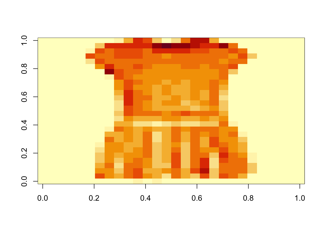
Let’s take a look at a few items and their labels.
<- 4 image (rotate_img (x_train[item_num, , ]))%>% filter (label == y_train[item_num])
# A tibble: 1 × 2
  label item
  <dbl> <chr>
1     3 Dress
Okay – I’m having a difficult time identifying these items. Can we train a sequential neural network to learn the classes?
<- keras_model_sequential (input_shape = c (28 , 28 )) %>% layer_flatten () %>% layer_dense (128 , activation = "relu" ) %>% layer_dropout (0.2 ) %>% layer_dense (10 )
Model: "sequential"
________________________________________________________________________________
 Layer (type)                       Output Shape                    Param #
================================================================================
 flatten (Flatten)                  (None, 784)                     0
 dense_1 (Dense)                    (None, 128)                     100480
 dropout (Dropout)                  (None, 128)                     0
 dense (Dense)                      (None, 10)                      1290
================================================================================
Total params: 101770 (397.54 KB)
Trainable params: 101770 (397.54 KB)
Non-trainable params: 0 (0.00 Byte)
________________________________________________________________________________
We have a model with over 100,000 parameters! Because random weights are initially set for each of these, we can use the model straight “out of the box” for prediction. We shouldn’t expect the network to perform very well though.
<- predict (model, x_train[1 : 2 , , ])
1/1 - 0s - 42ms/epoch - 42ms/step
#Predictions as a vector of log-odds
           [,1]      [,2]         [,3]      [,4]     [,5]       [,6]       [,7]
[1,] -0.3267654 0.5066797 -0.004953641 0.3215023 1.510471 -0.1182733 -0.3881088
[2,] -0.4342874 0.5235088  0.022825453 0.5869100 1.662138  0.1190307 -0.5709887
          [,8]      [,9]      [,10]
[1,] 0.2242094 0.7142845 -0.7938238
[2,] 0.4658616 0.3632336 -0.5920387
#Predictions as class-membership probabilities $ nn$ softmax (predictions)
tf.Tensor(
[[0.04941069 0.1137055  0.06816822 0.09448437 0.31025751 0.06086503
  0.04647076 0.08572475 0.13994041 0.03097277]
 [0.0412468  0.10748698 0.06514961 0.11452245 0.33562633 0.07172875
  0.03597672 0.10146587 0.09156915 0.03522733]], shape=(2, 10), dtype=float64)
Let’s define a loss function so that we can train the model by optimizing the loss.
<- loss_sparse_categorical_crossentropy (from_logits = TRUE )loss_fn (y_train[1 : 2 ], predictions)
tf.Tensor(3.331414385227533, shape=(), dtype=float64)
Before training, we’ll need to set the optimizer, assign the loss function, and define the performance metric. We’ll then compile the model with these attributes.
%>% compile (optimizer = "adam" ,loss = loss_fn,metrics = "accuracy"
Note that, unlike most actions in R, the model object is updated here without explicitly overwriting the object. This is because the underlying process is being completed in the Python Environment and then the transformed object is being passed back to R via reticulate.
Since the model has been compiled, we are ready to train it. Again, we won’t have to explicitly overwrite the model since the work is being done in Python and the objects passed back and forth.
%>% fit (x_train, epochs = 5 )
Epoch 1/5
1875/1875 - 1s - loss: 0.5350 - accuracy: 0.8106 - 1s/epoch - 697us/step
Epoch 2/5
1875/1875 - 1s - loss: 0.4013 - accuracy: 0.8545 - 1s/epoch - 624us/step
Epoch 3/5
1875/1875 - 1s - loss: 0.3687 - accuracy: 0.8659 - 1s/epoch - 625us/step
Epoch 4/5
1875/1875 - 1s - loss: 0.3457 - accuracy: 0.8730 - 1s/epoch - 584us/step
Epoch 5/5
1875/1875 - 1s - loss: 0.3331 - accuracy: 0.8769 - 1s/epoch - 591us/step
Now let’s evaluate our model performance.
%>% evaluate (x_test, y_test, verbose = 2 )
313/313 - 0s - loss: 0.3540 - accuracy: 0.8726 - 166ms/epoch - 530us/step
     loss  accuracy
0.3540442 0.8726000
We got 88% accuracy with a pretty vanilla and shallow neural network. There was only one hidden layer here, with 20% dropout. We didn’t tune any model hyperparameters and only trained over 5 epochs. We can see that loss was continuing to decrease and accuracy was continuing to climb from one epoch to the next here.
Since our model has been trained, we can use it to make predictions again.
<- model %>% predict (x_test[1 : 5 , , ])
1/1 - 0s - 21ms/epoch - 21ms/step
$ nn$ softmax (predictions)
tf.Tensor(
[[1.39241016e-05 7.38926365e-09 2.49174669e-06 2.23249155e-07
  1.45092461e-06 2.98859683e-02 4.71076834e-05 1.05881346e-01
  1.73178381e-05 8.64150163e-01]
 [6.49890895e-06 1.68627949e-11 9.96293891e-01 2.62089808e-09
  3.24826220e-04 6.88297559e-15 3.37477663e-03 6.34810896e-18
  4.90276462e-09 3.29867111e-16]
 [8.33620828e-10 9.99999984e-01 1.62753314e-10 1.17000810e-08
  3.23889926e-09 4.47634958e-15 3.01445034e-11 6.25351750e-17
  4.95748410e-11 5.67020142e-17]
 [1.93934026e-09 9.99998431e-01 1.05454079e-09 1.55390002e-06
  1.14922522e-08 3.24709571e-14 8.47580095e-10 1.09664119e-17
  4.92867328e-12 1.26356869e-14]
 [1.45070101e-01 2.72545607e-05 6.07397488e-02 1.46788816e-02
  1.03580528e-02 3.37159736e-07 7.67726429e-01 4.33174611e-08
  1.39876376e-03 3.87312010e-07]], shape=(5, 10), dtype=float64)
We can update our model so that it will provide class predictions rather than just the class membership probabilities.
<- keras_model_sequential () %>% model () %>% layer_activation_softmax () %>% layer_lambda (tf$ argmax)%>% predict (x_test[1 : 5 , , ])
1/1 - 0s - 31ms/epoch - 31ms/step
Now that we’ve trained an assessed one neural network, go back and change your model. Add hidden layers to make it a true deep learning model. Experiment with the dropout rate or activation functions. Just remember that you’ll need 10 neurons in your output layer since we have 10 classes and that the activation function used there should remain softmax since we are working on a multiclass classification problem. Everything else (other than the input shape) is fair game to change though!
Summary
In this notebook we installed and used TensorFlow from R to build and assess a shallow learning network to classify clothing items from very pixelated images. The images were \(28\times 28\) . We saw that even a “simple” neural network was much better at predicting the class of an item based off of its pixelated image than we are as humans.