Warning in plot_theme(plot): The `legend.pos` theme element is not defined in
the element hierarchy.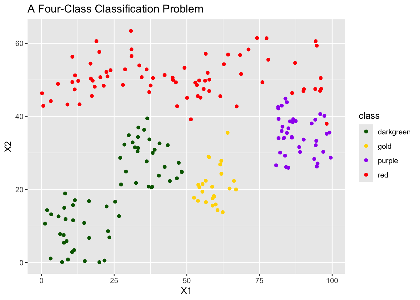
Purpose: In this notebook we’ll introduce decision tree models. These are another class of model which can be used in both the regression and classification settings. In particular, we note that
Decision tree models begin with all observations belonging to a single “group”. Within this single group/bucket, all observations would have the same predicted response. The fitting algorithms for decision trees then ask whether we could improve our predictions by splitting this bucket into two smaller buckets of observations, each getting their own prediction. The fitting algorithm continues in this manner until predictions are no longer improved or some stopping criteria is met.
Let’s see this in action by building a decision tree classifier on some toy data with four classes.
Warning in plot_theme(plot): The `legend.pos` theme element is not defined in
the element hierarchy.
Now that we have our data, let’s build a decision tree classifier on it.
Warning in plot_theme(plot): The `legend.pos` theme element is not defined in
the element hierarchy.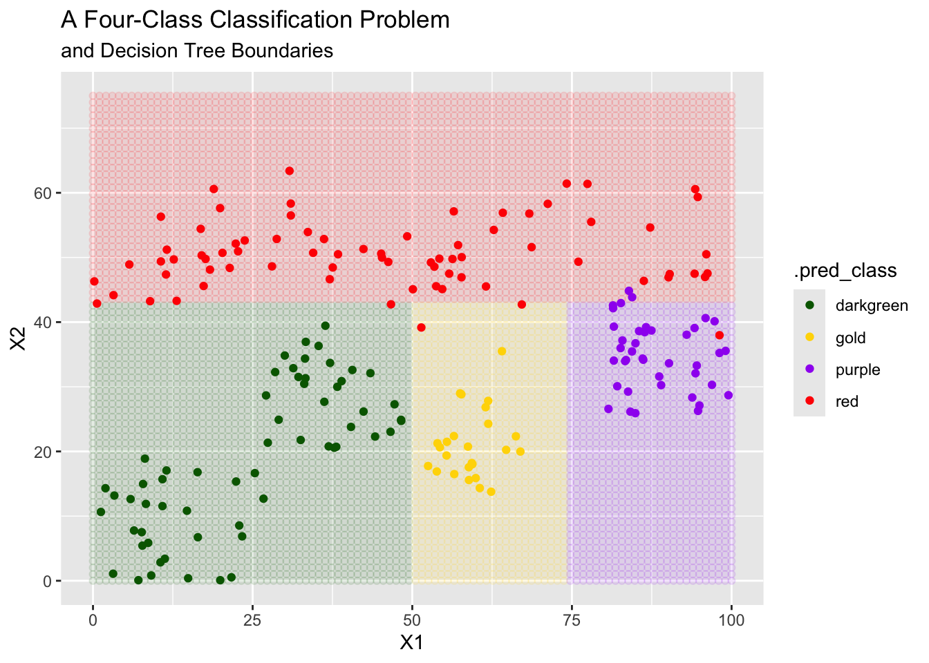
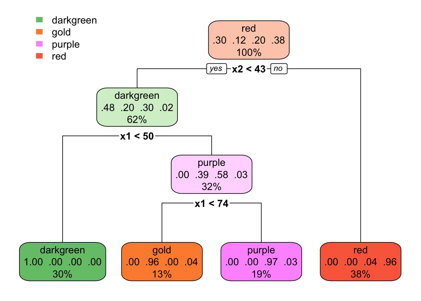
In the plot above, we see that the decision tree classifier seems to do quite well! The tree is asking yes/no questions about individual predictors (X1 or X2) which can be seen because the decision boundaries are perpendicular to those axes. In the plot below, we can see the actual structure of the decision tree.
Trees won’t always perform well, however. Indeed, if the optimal structure of the decision boundaries is not constructable via line segments perpendicular to the feature axes, we may end up requiring a very deep tree to approximate the decision boundary. A different model class is likely to be a better choice in these cases.
Consider the secondary toy dataset with two classes which is plotted below.
Warning in plot_theme(plot): The `legend.pos` theme element is not defined in
the element hierarchy.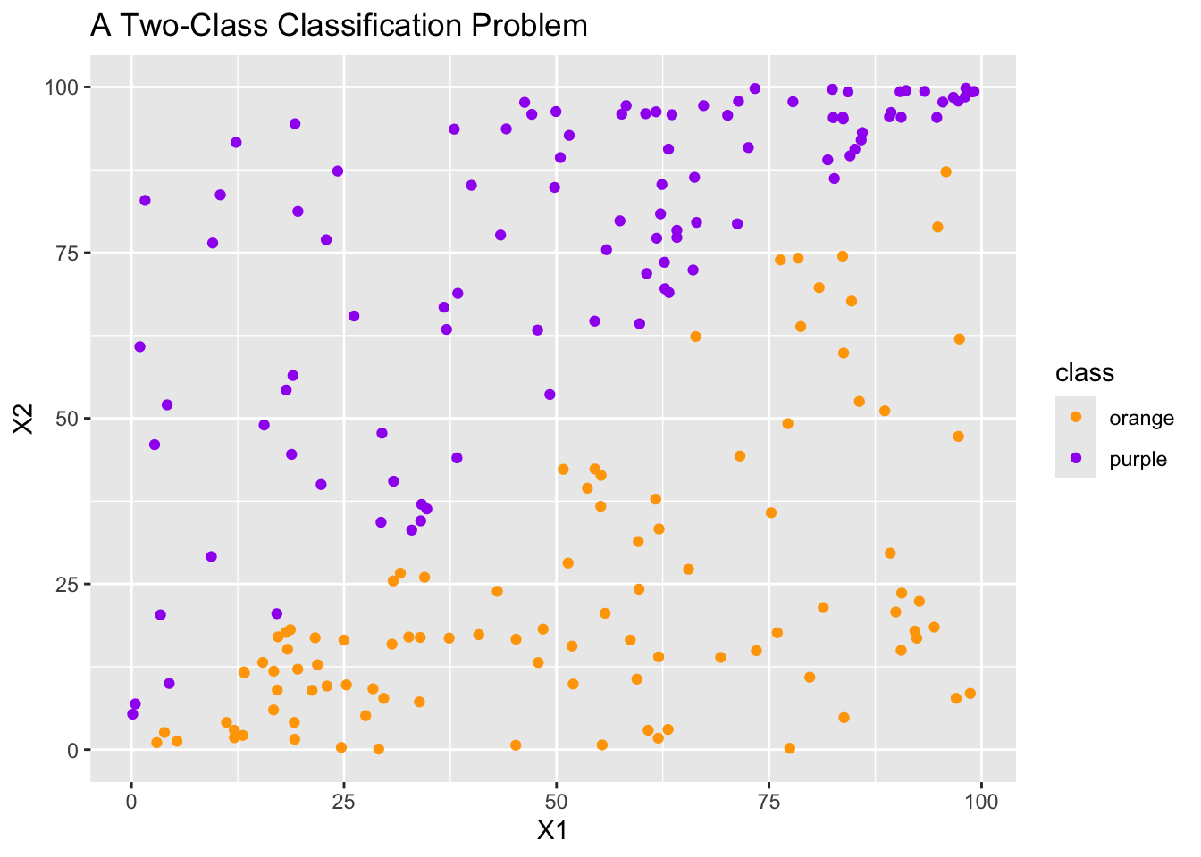
Now let’s try fitting a decision tree model to this data, as we did in the earlier example.
Warning in plot_theme(plot): The `legend.pos` theme element is not defined in
the element hierarchy.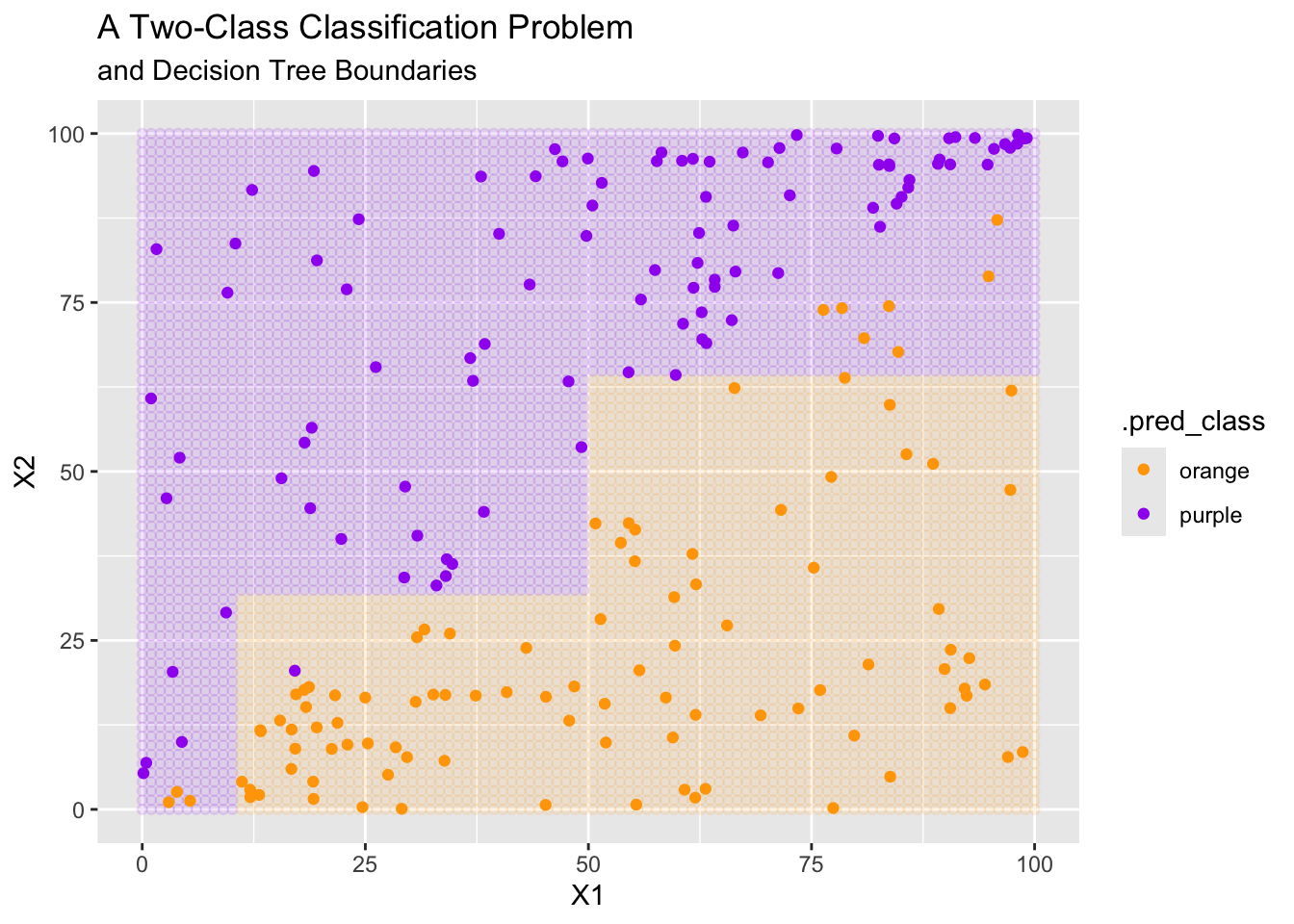
In the plot above, we see that the decision tree classifier is performing poorly, even though the classification problem should be quite easily! This is because the decision boundaries for a decision tree are perpendicular to those axes.
Knowing a bit about the structure of our data, what a likely decision boundary may look like, and which scenarios our model classes are best-suited for can be really helpful in making our modeling endeavors more efficient!
It will be useful to beware of the following regarding decision trees.
Decision tree models are enticed to overfit by their fitting process.
The deeper a tree, or the more end-nodes it has, the more flexible the model is.
We need to use regularization techniques to constrain our trees and prevent this overfitting.
{tidymodels} ecosystem has been built on a pit of success (rather than pit of failure) philosophy. The idea is that it should be easy to do the right thing, and difficult to do the wrong thing. For this reason, decision trees utilize some regularization by default to prevent overfitting.{tidymodels}A decision tree is a model class (that is, a model specification). We define our intention to build a decision tree classifier using
dt_clf_spec <- decision_tree() %>%
  set_engine("rpart") %>%
  set_mode("classification")
Decision trees can be used for both regression and classification. For this reason, the line to set_mode() is required when declaring the model specification. The line to set_engine() above is unnecessary since rpart is the default engine. There are other available engines though.
Like other model classes, decision trees have tunable hyperparameters. They are
cost_complexity, which is a penalty associated with growing the tree (including additional splits).tree_depth is an integer denoting the depth of the tree. This is the maximum number of splits between the root node and any leaf of the tree.min_n is an integer determining the minimum number of training observations required for a node to be split further. That is, if a node/bucket contains fewer than min_n training observations, it will not be split further.You can see the full {parsnip} documentation for decision_tree() here.
In this notebook you were introduced to decision tree models. This is a simple class of model which is highly interpretable and is easily explained to non-experts. These models mimic our own “If this, then that” decision-making style.