Warning: package 'kableExtra' was built under R version 4.2.2
Attaching package: 'kableExtra'
The following object is masked from 'package:dplyr':

    group_rows
#Read the penguins_samp1 data file from githubpenguins <-read_csv("https://raw.githubusercontent.com/mcduryea/Intro-to-Bioinformatics/main/data/penguins_samp1.csv")
Rows: 44 Columns: 8
── Column specification ────────────────────────────────────────────────────────
Delimiter: ","
chr (3): species, island, sex
dbl (5): bill_length_mm, bill_depth_mm, flipper_length_mm, body_mass_g, year

ℹ Use `spec()` to retrieve the full column specification for this data.
ℹ Specify the column types or set `show_col_types = FALSE` to quiet this message.
#See the first six rows of the data we've read in to our notebookpenguins %>%head(2) %>%kable() %>%kable_styling(c("striped", "hover"))
species
island
bill_length_mm
bill_depth_mm
flipper_length_mm
body_mass_g
sex
year
Gentoo
Biscoe
59.6
17
230
6050
male
2007
Gentoo
Biscoe
48.6
16
230
5800
male
2008
About Our Data
The data we are working with is a dataset on Penguins, which includes 8 features measured on 44 penguins. The features included are physiological features (like bill length, bill depth, flipper length, body mass, etc) as well as other features like the year that the penguin was observed, the island the penguin was observed on, the sex of the penguin, and the species of the penguin.
Interesting Questions to Ask
What is the average flipper length? What about for each species?
Are there more male or female penguins? What about per island or species?
What is the average body mass? What about by island? By species? By sex?
What is the ratio of bill length to bill depth for a penguin? What is the overall average of this metric? Does it change by species, sex, or island?
Does average body mass change by year?
Data Manipulation Tools and Strategies
We can look at individual columns in a data set or subsets of columns in a dataset. For example, if we are only interested in flipper length and species, we can select() those columns.
If we want to filter() and only show certain rows, we can do that too.
#We can filter by sex (categorical variables)penguins %>%filter(species =="Chinstrap")
# A tibble: 2 × 8
species island bill_length_mm bill_depth_mm flipper_le…¹ body_…² sex year
<chr> <chr> <dbl> <dbl> <dbl> <dbl> <chr> <dbl>
1 Chinstrap Dream 55.8 19.8 207 4000 male 2009
2 Chinstrap Dream 46.6 17.8 193 3800 fema… 2007
# … with abbreviated variable names ¹flipper_length_mm, ²body_mass_g
#We can also filter by numerical variablespenguins %>%filter(body_mass_g >=6000)
# A tibble: 2 × 8
species island bill_length_mm bill_depth_mm flipper_leng…¹ body_…² sex year
<chr> <chr> <dbl> <dbl> <dbl> <dbl> <chr> <dbl>
1 Gentoo Biscoe 59.6 17 230 6050 male 2007
2 Gentoo Biscoe 49.2 15.2 221 6300 male 2007
# … with abbreviated variable names ¹flipper_length_mm, ²body_mass_g
#We can also do bothpenguins %>%filter((body_mass_g >=6000) | (island =="Torgersen"))
# A tibble: 7 × 8
species island bill_length_mm bill_depth_mm flipper_l…¹ body_…² sex year
<chr> <chr> <dbl> <dbl> <dbl> <dbl> <chr> <dbl>
1 Gentoo Biscoe 59.6 17 230 6050 male 2007
2 Gentoo Biscoe 49.2 15.2 221 6300 male 2007
3 Adelie Torgersen 40.6 19 199 4000 male 2009
4 Adelie Torgersen 38.8 17.6 191 3275 fema… 2009
5 Adelie Torgersen 41.1 18.6 189 3325 male 2009
6 Adelie Torgersen 38.6 17 188 2900 fema… 2009
7 Adelie Torgersen 36.2 17.2 187 3150 fema… 2009
# … with abbreviated variable names ¹flipper_length_mm, ²body_mass_g
Answering Our Questions
Most of our questions involve summarizing data, and perhaps summarizing over groups. We can summarize data using the summarize() function, and group data using group_by().
Let’s find the average flipper length.
#Overall average flipper lengthpenguins %>%summarize(avg_flipper_length =mean(flipper_length_mm))
# A tibble: 1 × 1
  avg_flipper_length
               <dbl>
1               212.
#Single Species Averagepenguins %>%filter(species =="Gentoo") %>%summarize(avg_flipper_length =mean(flipper_length_mm))
# A tibble: 3 × 2
  species   avg_flipper_length
  <chr>                  <dbl>
1 Adelie                  189.
2 Chinstrap               200
3 Gentoo                  218.
How many of each species do we have?
penguins %>%count(species)
# A tibble: 3 × 2
  species       n
  <chr>     <int>
1 Adelie        9
2 Chinstrap     2
3 Gentoo       33
How many of each sex are there? What about by island or species?
penguins %>%count(sex)
# A tibble: 2 × 2
  sex        n
  <chr>  <int>
1 female    20
2 male      24
penguins %>%group_by(species) %>%count(sex)
# A tibble: 6 × 3
# Groups:   species [3]
  species   sex        n
  <chr>     <chr>  <int>
1 Adelie    female     6
2 Adelie    male       3
3 Chinstrap female     1
4 Chinstrap male       1
5 Gentoo    female    13
6 Gentoo    male      20
We can use mutate() to add new columns to our data set.
#To make a permanent change, we need to store the results of our manipulationspenguins_with_ratio <- penguins %>%mutate(bill_ltd_ratio = bill_length_mm / bill_depth_mm)#Average Ratiopenguins %>%mutate(bill_ltd_ratio = bill_length_mm / bill_depth_mm) %>%summarize(mean_bill_ltd_ratio =mean(bill_ltd_ratio),median_bill_ltd_ratio =median(bill_ltd_ratio))
# A tibble: 3 × 2
   year mean_body_mass
  <dbl>          <dbl>
1  2007          5079.
2  2008          4929.
3  2009          4518.
Data Visualization
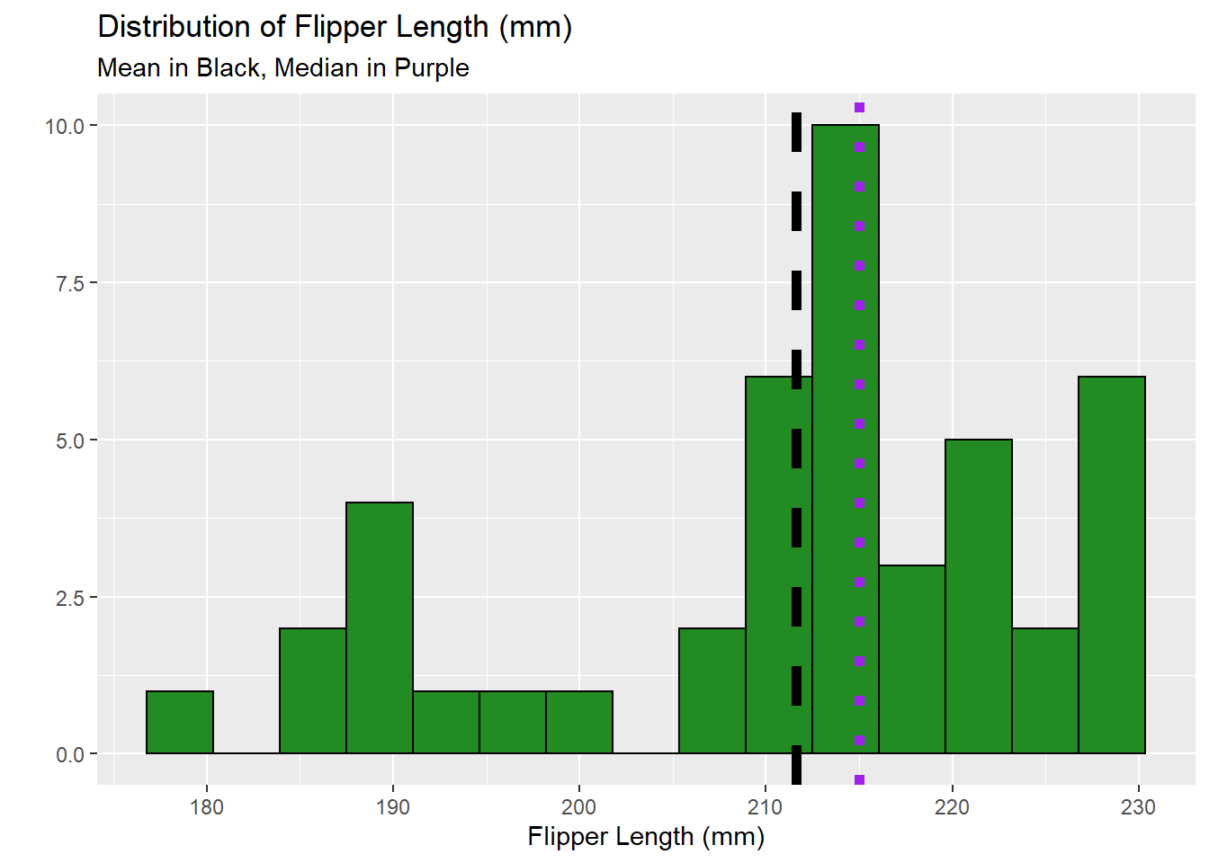
What is the distribution of penguin flipper lengths?
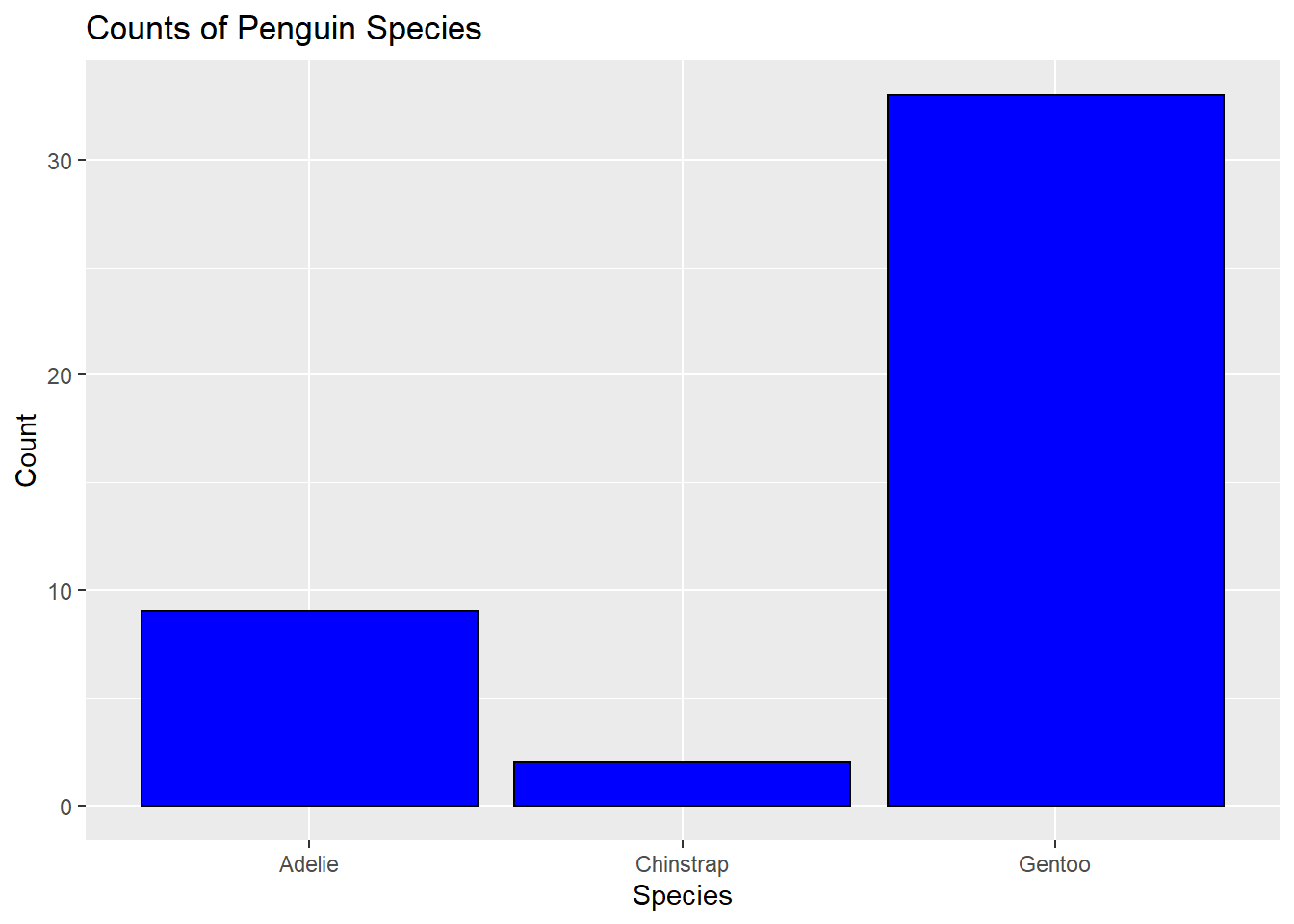
What is the distribution of penguin species?
Does the distribution of flipper length depend on the species of penguin?
penguins %>%ggplot() +geom_histogram( aes(x = flipper_length_mm), bins =15, fill ="forestgreen",color ="black") +labs(title ="Distribution of Flipper Length (mm)",subtitle ="Mean in Black, Median in Purple",y ="", x ="Flipper Length (mm)") +geom_vline(aes(xintercept =mean(flipper_length_mm)), lwd =2, lty ="dashed" ) +geom_vline(aes(xintercept =median(flipper_length_mm)), color ="purple", lwd =2, lty ="dotted" )
We will now look at the distribution of species.
penguins %>%ggplot() +geom_bar(mapping =aes(x = species), color="black", fill="blue") +labs(title ="Counts of Penguin Species",x ="Species", y ="Count")
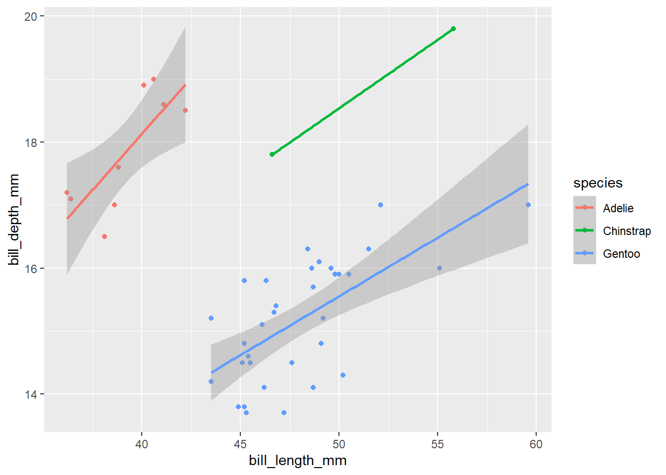
Let’s make a scatter plot to see if bill length is correlated with bill depth.
penguins %>%ggplot() +geom_point(aes(x =bill_length_mm, y = bill_depth_mm, color = species)) +geom_smooth(aes(x =bill_length_mm, y = bill_depth_mm, color = species), method ="lm")
`geom_smooth()` using formula 'y ~ x'
Warning in qt((1 - level)/2, df): NaNs produced
Warning in max(ids, na.rm = TRUE): no non-missing arguments to max; returning
-Inf